Convergence analysis of the finite difference solution for coupled Drinfeld-Sokolov-Wilson system

A crucial mathematical model called the Drinfeld–Sokolov–Wilson (DSW) system appears in a number of physical contexts, such as the quantum field theory and the integrable systems [1]. The coupled DSW system’s intricacy and the nonlinear characteristics make it a difficult subject for both the analytical and the numerical research [2]. The behaviour of complicated physical systems, such as DSW, has been studied widely using the numerical methods, such as the finite difference methods. The Crank–Nicolson scheme has become well-known among the different numerical techniques because of its time-stepping stability and the second-order temporal precision [3]. Although it has been applied to linear issues successfully, there are special difficulties once it is applied to coupled, nonlinear systems like DSW [4].Researchers have studied implicit techniques to solve coupled nonlinear systems in recent years [5]. Frequently, these techniques show improved stability characteristics, particularly for stiff problems. Based on this achievement, the Crank–Nicolson method, an interesting area for investigation, is applied to the DSW system along with the finite difference spatial discretization. The coupled DSW system’s finite difference solution will be thoroughly analyzed for convergence.

The mathematical model of the Drinfeld–Sokolov–Wilson system (DSW) as follows [6–12] :

∂u ∂v

^7 ⁺ Pv^T = ^{0 ,} ∂t ∂x

∂v    ∂ ³ v     ∂v     ∂u

+ q^l + ruTT + svTT = 0, ∂t    ∂x3     ∂x     ∂x which is represented by Drinfeld, Sokolov [9], and Wilson [13], represents a model of water waves. It has significant applications in fluid dynamics. Over years, a lot of numerical and analytical methods have been developed to solve these equations, including the

Adomian decomposition method [14], the Exp-function method [15], the improved F-expansion method [16], the bifurcation method [17], and the qualitative theory [18]. These methods offer various approaches to finding solutions for the system (1), (2). They have contributed to the understanding of its behavior and properties implicit. In this work, utilizing the implicit Crank–Nicolson approach. The efficacy and accuracy of this method will be investigated while offering the field brand-new insights.

1. Derivation of the Matrix Equation Using the FiniteDifference Method

A regular grid is introduced by defining the following discrete pair of points in the ( x, t ) plane:

xi = ih, i = 0,1,..., n, tj = jh, j = 0,1,...,m.

The discretized solution of equation (1) using IMFD method is:

„ j+1 _ jj -L pk 2 j Г, j+1 _ j++1 1 = fl uxi     uxi + 2hvxi Lvxi + 1 vxi-1J ”'

After arranging the above equation in terms of x i - 1 , x i , x i +1 we obtain:

(lj ) j⁺¹ C„7l^j+1        (? j ) ^j + ^{+ 1} =     (? j ) 1

^G 1 \v xij v xi — 1 ^{+ G} 2 u Xi ^{+ G} 3 v ^xi) v xi+1    [H u Xxi) J ,                ⁽³⁾

where

G 1 (v Xi ) = - phv Xi , ^G 2 = 1 , ^G 3 (v Xi ) = phv Xi , H (u Xi ) = ^u j_xi .

Then

^G (v j ) { ^{u j +}\^{V j +1} } = {H(u Xi )} for i = ^{2 ,} 3 ,...,n ^- 1 .              (4)

For i = 1 we have:

G,j1 +G3 (j) • vX+1 = {H Hi)} and for i = n :

G1 ( j    • v j+12 + G₂ u j+1 = { H (ul) } .

xn -      xn -         xn           x

Note that the definitions of Gi fvj.,-, G₂ , G₃ fv ^jJ and H fu ^jJ depend on vj and u ^j ,.

xi                 xi                 xi                     xi          x i

Where G ( v j ) is the tri-diagonal matrix:

' _ G 2      G 3 ( v X2 )  _ 0         0     0  0        •            •            0     ' G 1 (v X2 )       G ,      G 3 (v X3 )       0      0  0         •              •              0 0      G 1 (v X3 )       G 2      G 3 (v X4 ) 0 0         •              •              0 0                0                 •                 •           •     0             •                     •                     0 0                0                0                 •           •    •             •                     •                     0 •                       •                       0                     0               •      •                 •                            •                            • .                       .                       0                     0               •      •                 •                            •                            • 0          0          0          0        • • G 1 (v Xn - 1 )        G ,        G 3 (v Xn - , ) 0          0          0          0        • •         0        G3 (vj„_2)        G2 xn - 2

jd Л j+1 j+ +1 j+⁺¹ j+⁺¹ j+⁺¹ j+ +1 } T

And { v } — ^v xi , u xi , v x2 , u x2 . . . , v xn - 1 , u xn - 1 J

I (i j ) 1 ІН (i j +1 1      (i ij⁺¹ 1          (i ij⁺¹ 1 }

I H \u ) J ^— lⁿ \u x1 ) , H \u x2 J , . . . , ^H Vu xn - 1 J J

By the same approach for equation (2) we obtain:

j +1 xi

-

k

+ rv X +¹

v ^j

— + q- ujxi+1

(v j ⁺¹ v xi +2

-

2 h

- 2 v X ++11 + 2 v X + - 11

2 h ³     ₊₁

u xi - 1         j    v xi +1

------ ) + s^U Xi I ------

j⁺1 1 v xi - 2) +

-

2 h

j +1 v xi - 1

‘Р (i j^{+1 1} T’P   (i j 1 (i j ⁺¹ 1    ‘     (i j 1 (i j⁺¹ 1

E ¹ vxi - 2/ ⁺ E ² uxxi) vxi - 1/ ⁺ E 3 uxxi) vxxi ) ⁺

+'^E 4 ( ^U Xi 1 (v X+11 1 ^- ‘ E 5 (v X+12 1 ^— vj ⁽ xi ) .

For i — 1 , 2 ,..., n — 1, where

‘ ^{E 1 — —} ■ ’

‘ E 2 (ux1 — ( T ) — Th j , _{′ j}           rk _j sk _j

^E 3 (u xi) ^{— 1} + ^ (u xi+1) ^— 2 h (u xi - 1/ , ‘ ^E 4 (^U Xi 1 ^{— —}'^E 2 (^U Xi 1 , ‘ ^E 5 ^{— —} ‘ ^E 1 , ^F Kv Xi 11 ^— v x i .

Now equation (4) becomes in following algebraic matrix equation:

^′ E u i ^j · v i ^{j +1}

} — {F (vXi)},

where ^′ E u _i is the tri-diagonal matrix:

we proved that was

′ E 3 u j xi	— E 2 (иіі1	- ′ E 1	0	0	0	·	·	0
′ E 1	′ E 2 u j xi	′ E 3	E j 1	- ′ E 1	0	·	·	0
0	′ E 1	′ E 2 u j xi	′ E 3	— E 2 ( u xi 1	- ′ E 1	·	·	0
0	0	·	·	·	0	·	·	0
0	0	0	·	·	·	·	·	0
·	·	0	0	·	·	·	·	·
.	.	0	0	·	·	·	·	·
0	0	0	0	′ E 1	Ette 1	′ E 3	E 2 (u xi 1	- ′ E 1
0	0	0	0	·	·	′ E 1	′ E 2 u j xi	′ E 3

Now, the existence of the solution of the matrices equations was obtained from equation (3) and (4) respectively.

Theorem 1. The solution of the matrices equations

• (i)    G ( v j ){^ ⁺¹ ,_И ’⁺¹ } — { H ( j )} ;

• (ii)    ‘ E (u j ){v j⁺¹ } — { F (v j )} exist.

Proof. (i): Let j E N be fixed, consider the following iteration:

G (v j — 1 ) {u j⁺¹ ,v j⁺¹ } = {H «)} , V i E N.

Where v 0⁺¹ = v j , by subtracting the last equation from

G (v j ){u j⁺¹ ,v j⁺¹ } = { H (u ii )} .

we have

G (vj — 1) {u j⁺¹ , v j⁺¹} - G ( v j) {u j⁺¹ ,v j⁺¹} = 0 , G_(v j ) {u j⁺¹ _! j¹ } - G (v j- ) {u j⁺¹ v j⁺¹ } =

G (v j ) [{u j⁺¹ , v j⁺¹ } - {u j⁺¹ , v j⁺¹ }] = [ G (v j - 1 ) - G (v j )] • {u j⁺¹ , v j⁺¹ } ( x , ) .

The k -th element of the right hand side of equation (6)

n — 1

£ ( c ks (^{v j} — 1 ^{( x} k ) ^- c k,s (^{v j ( x} k ) ^{( x} s ) ) • {u j ^{+ 1 ,v j + 1} } ^{( x} s ) .

s=1

By the mean value theorem:

n — 1 n — 1

££ c ks (^v j * ^{( x} k ) ) _{X L} • (v j — 1 ^{( x} L ) ^{- v} j ^{( x} L ) ) • {u i ⁺ \ ^v j⁺¹ } ^{( x} S ) .

s=1 L=1

( x k ) is between v j _{— 1} ( x k ) and v j ( x k ) and ^k,_s (v j * ( x k ) ) xj

where the value of v _i ^j ∗

represent

the partial derivatives of (c k,_s (v j * ( x k )) with respect to v j * ( x _L ).

Now the right hand side of equation (5) becomes:

n — 1 n — 1

EE '

s=1 L=1

where ‘ Q (u ^{j +1} ,v j⁺¹ , u ^j * )

is the following matrix:

n=1

^E {^{u j +1 ,v} j⁺¹ } c 1,s (^v j * ^{( x} k ) ) x 1 s=1

n=1

E {u ,^{+1 ,v j +1} } ^c 2,s (v j ^{( x} k ) ) x 1 s=1

n=1

E ■ ⁺¹ ,v j⁺¹

s=1

n=1

E {u j⁺¹ ,v j⁺¹

s=1

} c , (v j * ⁽ x k )) X n - 1

^{} c} 2, ^(v j * ^{( x} k ^

n=1                                               n=1

s=1                                             s=1

Since c1,svj* (x1), s = 1,2,..., n — 1, contains only vj* (x1) and vj* (x2) hence n-1

'01,1 (vj*) = £ {uj+1,vj+1} (xs) c1,s (uj* (x1))X1, s=1

' ⁰ 1,1 (v j *) = u i ^{+1 (} x i ) c i,i (^{v j} * ⁽ x i )) _{x 1} + ^{v j +1 ( x} 2 ) c i,2 (^u ) . ^{( x} 1 )) _{x 1} ,

' 0 1,1 ( v* ) = u i⁺¹ • (0) + (2k) • v j+1 ( x 2 ) <

(th) •^{v j +1 ( X 2 )} |<^{€ 1} ,

n - 1

'01,2 (vj*) = £ {uj + 1,vj + 1} (xs) c1,s (uj* (x1 ))x2 , s=1

'01,2 (vj*) = ui+1 (x1) c1,1 (vj* (x1))x2 + vj+1 (x2) c1,2 (ui* (x1))x2 , '01,2 (vj*) = uj+1 (x1) • (0) + vj+1 (x2) • (0) = 0 < €2, for some €1, €2 < 1.

(2h)

Let r =

, since k and h are both small, we can make r bounded by letting k be sufficiently small, vj+1 is bounded, then '01,1 (vj*) is bonded by small numbers, therefore, all the elements in the row of the matrix '0 are zero expect the first element, which is sufficiently small.

Similarly we can find c _{n -1} ,_s v j * ( x _{n -1} ) only contains v j * ( x _{n -2} ) and v j * ( x _{n -1} ), s = 1 , 2 , . . . , n — 1, which implies that:

' 0 n - 1,L (v j *) = 0

if L = n — 1.

If L = n — 1 we have

'0n-1,n-1 (vj.) = vj + 1 (Xn-2) Cn-1,n-2 (vj* (Xn-1)k  , + xn-1

+ U j ⁺¹ ( X n - 1 ) C n - 1,n - 2

(v ^j * ( x n - 1 )) x n - 1

' 0 n - 1,n - 1 (v j * ) = | kv j⁺¹

( X n - 2 ) + U j⁺¹ ( X n - 1 )(0) ,

⁰ n - 1,n - 1 (v i * ) <

3 k

2 h

|v ^{j +1} ( X n - 2 ) | < € 4 .

In general we have ' 0 k,k (v j *) = 0 for any values of k, therefore the matrix ' 0 (v j *) has the following form:

' ' 0 1,1 (v j * )          0              0        0 0 0 .         .                0       ' 0         ' 0 1,1 (v j * )          0        0 0 0 .         .                0 0              0         ' 0 1 , 1 (v j * ) 0 0 0 .         .                0 0                    0                  ’ .             . . 0 .             .                      0 0           0           0       ..... 0 .          .           0      0   ...      .          . .          .           0      0   ...      .          . 0              0              0        0 . . 0 ' 0 1,1 (v j * )          0 0              0              0        0 . . 0        0         ' 0 1 , 1 (v j * )

,

where the non-zero elements are sufficiently small. Thus, the norm of the matrix ' Q, which was defined by sup _{x e} R n - i || ' Q (u j⁺¹ , v j⁺¹ , v j *) || was small and bounded. Now, what remains is to show that ' Q is invertible and is bounded away from zero. The matrix ' Q is positive definite and is bounded away from zero, since we can choose k, h, p, q, r and s can be chosen such as the diagonal of the matrix is positive and hence invertible. By this, the proof of part is completed (i).

(ii): ‘ E (uj) {v^ ¹} = {F ( v j ( x i )) } as in part (i) note the following iteration

‘E (uj—1) {vj+1} = {Fuj (x,)} Vi G N, where u^ = uj+1. By subtracting the last equation from

' E (u j ₊ 1 ) {v j⁺¹ } = { Fv j ( x , ) } , Vi G N.

We have

'E (uj—1) {vj+1} — ‘E (ujЖ11} =0, by adding and subtracting 'E (uj) {vj1}, we obtain

' E ( u j ) {v j⁺¹ } - ' E ( u j ) {v j⁺¹ } = ' E (u j - 1 ) {v j⁺¹ } - ' E (u j ) {v ^{j +1} } , ' E (u j)    + — v j⁺¹} = [' E (u j - 1) — ' E (u j)] {v j⁺¹} ( x , ) ,

the k -th element of the right hand side of equation (6)

n — 1

£ (^e k,s ^u j — 1 ^{( x} k ) - ^e k,s ^u j ^{( x} k ) ) {^{v j + 1} } ( x s ) .

s=1

By the mean value theorem:

n — 1 n — 1

£ £ (^j (xk))xL • (uj—1 (xL) - uj (xL)) • {vj + 1} (xs) , s=1 L=1

where the value of u j ( x _k ) is between u j _{— 1} ( x _k ) and u j ( x _k ) and (e _k,_s (u j * ( x _k )) )x represents the partial derivatives of e _k,s (u j * ( x _k )) with respect to u j * ( x _L ) . Now the right hand side of equation (6) becomes:

^{£ £} {v j⁺¹ } ( x . ) B k* (u j * ( x k ) ) x _L • (u j — 1 ( x l ) s=1 L=1

where 'E vv+⁺\u**_i*'} is the following matrix:

E” ¹ {v j⁺¹ } B 1.‘ (u j - ( x k ) ) _{x i}    ....

EZ 1 {v j⁺¹ } B ₂* (u j - ( x k ) ) x 1    ....

En= {vj ^{+ 1}} B n — 1,. (uj - ( xk))x 1

• ^{- u} j ^(xL ) ) = '^E (NX.Uj. ) • {^{u j} — 1 ^{,u j} } ,

E n=1 {v j⁺¹ } B 1,s ( u j - ( x k ))„ , 1

ES 1 {v j⁺¹ } Bx . (u j . ( x k ) ) x n - i

.

. ..

.

.

.

E2 {v j⁺¹ } B „ — 1. (u j * ( x k ) ) , . -__

Since e 1,s j* ( x 1 )) , s = 1 , 2 ,..., n — 1 , only contains j ( x 1 ) and u j ( x ₂ ), hence

‘ E 1,1 (u i - ) = E           ( x . )           ( x 1 )) x i ),

‘ E 1,1 (u j - ) = V +1 ( x i ) (e_U ( u j ( X 1 )) x i ) +

+ v ^{+1 ( x} 2 ) (^e 1,2 ^{( u j} * Ык ) + ^{j ( x} 3 ) (^e 1,3 ^{( u j} * ^{( x} 1 )k ) , ' ^E 1,1 ( j ) = ^ 1,2 ( j ) • ⁽⁰⁾ + v j^{+1 ( x} 2 ) • ^ + v j^{+1 ( x} 3 ) • ⁽⁰⁾ .

According to the properties of absolute value we have:

' E 1,1 ( j ) — T • h

j

^{( x} 2 ) I < £ 1 ,

' E 1,2 (u j - ) = E . ( x . ) в 1,. (u l ( x 1 ))_M , ' E 1,2 (u i - ) = V ⁺¹ ( x 1 ) в 1,1 (u i - ( x 1 ) ) , ₂ +

+ ^{v j + 1 ( x} 2 ) ^в 1,2 ^{j ( x} 1 ⁾ ) x 2 + ^{v j + 1 ( x} 3 ) ^в 1,3 ( j ^{( x} 1 ) )

^x 2 ^,

• j ⁽ x 1 ^{) |}< £ 2 ,

k

' E 1,2 C j ⁾ = ^{j (} x 1 ) • 2 h + ^{j (} x 2 ) • (0) + V ^{j +}

( x 3 ) • (0) —

for some £ 1 and £ 2 <  1.

' E 1,3 (^{u j} -) = v j⁺1 ^{( x} 1 ) ^в 1,1 j ^{( x} 1 )) _x 3 +

+ vj + 1 (x2) в1,2 j (x1))   + vj + 1 (x3) в1,3 j (x1))a. , x3                                   x3

' E 1,3 ( j ) = v j ⁺1 ^{( x} 1 ) • (0) + v j ⁺1 ^{( x} 2 ) • (0) + j^{1 ( x} 3 ) • (0) , ' E 1,3 ( j ) = ⁰ < ^£ 3 .

Let r = —, since к and h are both small, r can be bounded by letting к be sufficiently h small , vj+1 is bounded then ′E1,1 uij∗ and E1,2 uij∗ are bounded by small numbers. Similarly en-1,. (uj (xn-1)) only contains j* (xn-3)) , (uj- (xn-2)) and (uj (xn-i)), s = 1,..., n — 1, implies that:

' E n - 1,L ( j ) =0 if L = n — 2 , n — 1 ,

^E n — 1,n - 2 (u i » ) —

k

2 h

j+1 v _i

( x n - 1 ) ¹< £ 5 .

In the same way

^E n — 1,n — 1 (^u i - ) < ^£ 6

for some £ 5 and £ 6 <  1.

Now we have к (xk-2), к (xk-1) , к (xk) , к (xk+1)

and u ^j ( x _{k +2} ) in B k^ u j ( x k ), where к = 1 , n — 1 , s = 1 ,...,n — 1 , i = 3 , ...,n — 2 .

Then ‘ E k,i (u j .) = 0, if L = K - 1 ,K, K +1 and ^′ E k,k - 1 u i ^j ∗ ^{<  ǫ} 7 ^, ‘ Ek,k (ui* ) < ^ 8 , ^′ E k,k +1 u i^j ∗ < ǫ 9 , ^′ E k,k +2 u i^j ∗ < ^ǫ 10 for some e i <  1 , and any i.

Therefore the matrix ^′ E u _i ^j ∗ has the following form

′E1,1  uij∗ ′E1,2 uij∗ 0 0 0 0·                                               · 0 0 ‘ E2,2 j ) ‘ E (j ) · ‘E24 j ) · 0 0 · · 0 0 0 · 0 · · 0 0 0 · · · 0 · · 0 0 0 0 · · · · · 0 · · 0 0 · · · · · · · 0 0 · · · · · 0 0 0 0 0 ‘E j ) En-2,n-3 ui∗ En-2,n-2 ui∗ 0 0 0 0 0 · · 0 En-1,n-2 ui∗ En-1,n-1 ui∗ when the nonzero elements in the matrix ′E uij∗ are small, then the norm of the matrix which is determined by supxeR n — 1 ^‘E Vj++1, u++1) Ц, is bounded and small.Now, it is important to show that the invertible and it is bounded away from zero. Thus, the matrix is bound away from zero and it has a positive definite value because we can select k, h, p, q, r and s can be selected such that the diagonal of the matrix is positive and that in every row, the magnitude of the diagonal entry in arrow is greater than the total of the magnitudes of all the other (non-diagonal) entries in the row. The proof of part (ii) is complete.

• 2.    Numerical Experiments

In this section, an applied example will be taken to employ the IMFD method so to obtain numerical solutions for the system which is described by the following equations [15]

du +*s -"■

∂v    ∂ ³ v ∂u

∂u

^{+ 2} Ғ з ⁺ R^-v ^{+ 2u}R^— = ⁰

∂t    ∂x ³ ∂x ∂x

with initial conditions

u ( x, 0) = 3 sech ² ( x ) ,

v ( x, 0) = 2 sech( x ) .

and analytic solution of the (DSW) [8]

/          3c

u ( x, t ) = у sech

(I(x

— ct

^{— a)}^ ,

v ( x, t ) = c

^sech(yi^{( x}

—

ct — a )) ,

where x and t are independent variables, u = u ( x,t ) ,v = v ( x,t ) and [ — 20 , 20] is the solution region ( a, c E R).

In order to compare the numerical results with the analytical solution, we will utilize error measurer:

ABSE = | u i ( x, t) — u ( x, t ) | ,

_MSE = J lnLo ^{( u} i ^{( x,t )} - ^{u ( x,t )) 2}

• У            n

are used in which u,v,u _n and v _n represent analytic and numerical solutions respectively.

The numerical solution will be given from the IMFD method in this part and be contrasted to them with the (DSW) equation’s analytical solution. It is important to note that the system’s analytical solution will be utilized as a standard for comparison. In all computations, a = 0 , c = 2 , — 20 <  x <  20 , n = 51 , m = 51 , h = 2 ,k = 0 , 001 and t =1.

Table 1

Compare the IMFD method with the analytical solution for (DSW) for u

x	Exact -u	IMFD -u	ABSE
-20	0,000000000000000	0,000000000000000	1 , 80205E — 08
-18	0,000000000000003	0,000000000000008	8 , 92562E — 08
-16	0,000000000000151	0,000000000000421	4 , 42086E — 07
-14	0,000000000008264	0,000000000022967	2 , 18958E — 06
-12	0,000000000451208	0,000000001252916	1 , 08431E — 05
-10	0,000000024635106	0,000000068126298	5 , 36582E — 05
-8	0,000001345030896	0,000003653660151	2 , 64594E — 04
-6	0,000073435316301	0,000186806182197	1 , 28251E — 03
-4	0,004006803508809	0,008317084833155	5 , 73678E — 03
-2	0,211136676642920	0,259362920446189	1 , 79981E — 02
0	2,999988000032000	2,895253604333530	5 , 67486E — 03
2	0,212771304327143	0,261528044421427	4 , 95361E — 02
4	0,004038964825597	0,008512274892351	1 , 37328E — 03
6	0,000074025147763	0,000193114247779	1 , 58509E — 02
8	0,000001355834296	0,000003796067950	5 , 30780E — 03
10	0,000000024832977	0,000000070918670	1 , 19785E — 03
12	0,000000000454832	0,000000001305033	2 , 47619E — 04
14	0,0000000000008331	0,000000000023925	5 , 02362E — 05
16	0,000000000000153	0,000000000000438	1 , 01525E — 05
18	0,000000000000003	0,000000000000008	2 , 05015E — 06
20	0,000000000000000	0,000000000000000	4 , 13935E — 07
MSE			1 , 06320 E — 04

Comparing Tables 1 and 2, it can see that the IMFD method quantity of MSE is the numerical results that proved the numerical solution was close to the real solution at different values of time. The following Figs. 1 and 2 represent the exact solution and the numerical solution and IMFD method for each of u and v at a = 0 , c = 2 , — 20 <  x <  20 , n = 51 , m = 51 , h = 2 , k = 0 , 001 and t = 1.

Table 2

C ompare the IMFD method with the analytical solution for (DSW) for v

x	Exact -v	IMFD -v	ABSE
- 20	0,000000008228142	0,000000008244614	1 , 20494E - 06
- 18	0,000000060798201	0,000000060919919	2 , 68240E - 06
- 16	0,000000449241317	0,000000450140699	5 , 97354E - 06
- 14	0,000003319469294	0,000003326114891	1 , 33126E - 05
- 12	0,000024527744835	0,000024576850191	2 , 97147E - 05
- 10	0,000181236882197	0,000181599761125	6 , 65246E - 05
- 8	0,001339169342398	0,001341852660690	1 , 49589E - 04
- 6	0,009895137950933	0,009915068470069	3 , 35986E - 04
- 4	0,073091755201340	0,073243266329343	7 , 13916E - 04
- 2	0,530580407532380	0,531539548105092	9 , 55317E - 04
0	1,999996000006660	1,987099645410510	2 , 99119E - 03
2	0,532630333755214	0,531540621903467	1 , 28692E - 02
4	0,073384510859781	0,073243356048958	6 , 96227E - 03
6	0,009934797281164	0,009915070988441	1 , 90480E - 03
8	0,001344536746210	0,001341852713397	7 , 02059E - 04
10	0,000181963281553	0,000181599762127	3 , 12933E - 04
12	0,000024626052298	0,000024576850209	1 , 43159E - 04
14	0,000003332773763	0,000003326114891	6 , 51232E - 05
16	0,000000451041881	0,000000450140699	2 , 94484E - 05
18	0,000000061041881	0,000000060919919	1 , 32720E - 05
20	0,000000008261120	0,000000008244614	5 , 97180E - 06
MSE			6 , 73200 E - 04

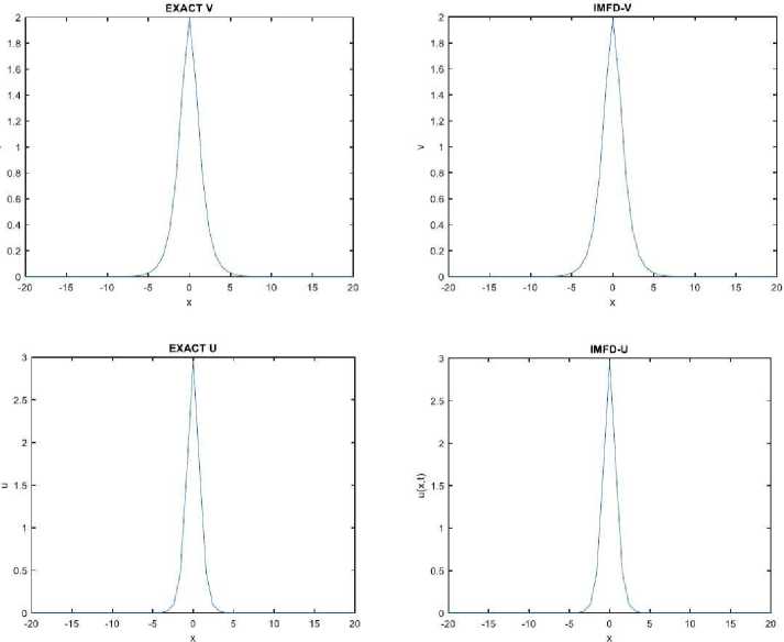
Fig. 1 . Represents 2D solutions of EXACT and IMFD method for each of u and v

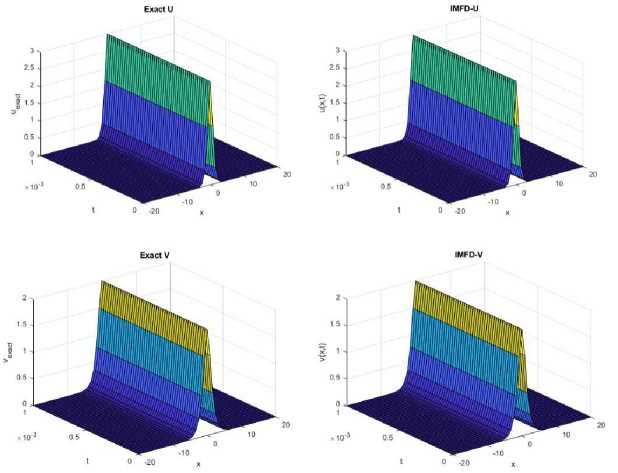
Fig. 2 . Represents 3D solution of EXACT and IMFD method methods for each of u and v

These findings highlight the effectiveness of the IMFD method approach in effectively handling the nonlinearities of the equation effectively, resulting in precise and efficient solutions. Furthermore, the comparison of the results obtained from the IMFD method and the exact solution.

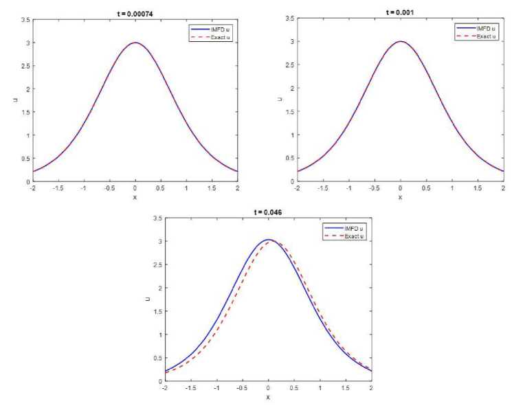
Fig. 3 . Comparison IMFD method and Exact solutions for u and v with different times

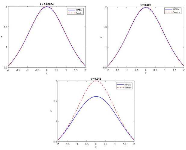
Fig. 4 . Comparison IMFD method and Exact solutions for u and v with different times

Conclusions

The basic idea of this paper was to demonstrate that using the IMFD method to solve (DSW) systems is feasible and it has even been proposed as a theory in this regard. This was done because the method was developed from a system of nonlinear algebraic equations. It was also shown in this paper’s concluding section that using the method of fixed point iteration to solve nonlinear systems yields acceptable results in addition to its simplicity as far as its use is concerned. The numerical solutions of the examples in the Tables 1,2 and Figures 1 – 4 show that, the IMFD method produce results that are closer to the exact solutions for different values of t . The ABSE and MSE were used to compare the numerical results.

Acknowledgments. The research is supported by the College of Computer Sciences and Mathematics, University of Mosul, Republic of Iraq.