Cost-effective Robotic Arm Simulation and System Verification

Published Online on April 8, 2024 by MECS Press

The advent of digital manufacturing within the Industry 4.0 framework has ushered in a transformative era characterized by the integration of communication systems, big data handling, Artificial Intelligence (AI), and the Internet of Things (IoT) into modern manufacturing technologies. This convergence is evident across various manufacturing domains, including conventional and non-conventional machining, additive manufacturing, and robotic manufacturing. The integration of these technologies aims to propel the manufacturing industry towards a greener, more sustainable, safer, and cost-effective production environment. One powerful tool that has emerged in this landscape is robotic simulation, which plays a pivotal role in manufacturing and education [1-5].

Existing literature underscores the significance of robotic simulations in addressing diverse aspects of the manufacturing process, such as energy consumption, path planning, design, programming, and error identification [610]. Notable studies include Bres et al.'s model-based framework for simulating and optimizing friction stir welding using robots [11], Xiao et al.'s STEP-compliant model for industrial robots [12], and Raza et al.'s exploration of integrating CAD modeling and finite element analysis for optimal robotic arm design [13]. Additionally, MATLAB has been utilized for both forward and inverse kinematics analysis and 3D representation of robot models [14].

Manufacturing automation, particularly in the context of intelligent manufacturing, has significantly benefited from the creation of virtual worlds or digital twins [15-17]. Bilberg and Malik [18] demonstrated the simulation of a robotic assembly cell as a digital twin, promoting the flexibility of human-robot work teams. Other studies explore the digital twin creation of multi-robot manufacturing environments [19], production system reconfiguration in flexible assembly lines [20], and the application of mixed reality for safety awareness in human-robot collaboration [21]. These endeavors underscore the potential of digital twins in training operators, achieving real-time monitoring, and optimizing manufacturing processes.

Despite these advancements, there remains a need for further research and the development of updated simulation models, especially in the realm of robotics, which is widely implemented across various industries [21-23]. This paper addresses this gap by presenting the design and construction of a 5 DoF robotic arm manufactured entirely with 3D printing technology. The robotic arm is seamlessly integrated into a simulator system using appropriate software and CAD models. Our approach, grounded in cost-effective methods and innovative design processes, contributes to the evolving landscape of robotic simulations and digital twins. Through a detailed kinematic analysis, we demonstrate the accuracy and efficacy of our digital platform in replicating real-world robotic systems.

In summary, this introduction highlights the ongoing advancements in digital manufacturing, the pivotal role of robotic simulations, and the existing gaps in the current scientific discourse. Our research aims to bridge these gaps by providing a cost-effective solution for the design and implementation of a 5 DoF robotic arm, presenting a valuable addition to the field of robotic simulations and digital twins.

2.    Related Works

It is evident that robotic simulations are applied widely in the industry, focusing on the energy consumption, path planning and design, programming, as well as error identification [6–10]. Bres et al. [11] established a model-based framework for the simulation, analysis and optimization of friction stir welding using robots, focused on the assembly of aluminium aircraft components. Xiao et al. [12] presented a STEP-compliant model for industrial robots, for data exchange between computer aided systems and robot off-line programming systems. This method can be used to represent most resources involved in a robotic manufacturing system, including the robots’ kinematic and dynamic behaviors. Raza et al. [13] investigated the feasibility of integrating tools such as CAD modeling and finite element analysis, for the optimum robotic arm design. The authors used Robo-Analyzer for the inverse kinematics analysis. Another software system utilized for the robotic design is MATLAB. Barakat et al. [14] used MATLAB for both the forward and inverse kinematics analysis, and for the 3D representation of the robot model.

Manufacturing automation and intelligent manufacturing in general seem to benefit from the generation of virtual worlds, fact that is proved by studies that are related to several cases of manufacturing technologies [15–17], including recent advances as well, such as the additive manufacturing. Bilberg and Malik [18] presented a simulation as a digital twin of a robotic assembly cell, promoting the flexibility of a human-robot work team. Similar studies are found in the literature for the digital twin creation of multirobot manufacturing environment [19], with an aim to efficiently train operators, achieve real-time monitoring and optimization. Production system reconfiguration in flexible assembly lines [20], such as the ones found in a car factory, can be achieved with the creation of a digital infrastructure involving sensor data, CAD models and dynamic communication. Choi et al. [21] proposed an approach with mixed reality for safety awareness with deep learning and DT generation, finding application on the human-robot collaboration. Safety awareness between human-robot interactions in manufacturing environments, as well as the optimization of the robotic operability [21–23], is a widely studied topic. Since robotics are implemented in many industries and especially in manufacturing, more research is required and a wider number of updated simulation models need to be developed.

This paper presents the design and construction of a 5 DoF robotic arm that was entirely manufactured with the help of 3D printing technologies and then integrated in a simulator system, with the help of appropriate software and the equivalent CAD models. Similar kinematic analysis studies for various robotic applications [24,25], are based on the design and simulation techniques.

3.    Robotic Arm Design and Digital Twin Implementation

The robotic arm was designed and its individual parts were printed on a 3D printer. It was assembled, and with the help of the appropriate motors and drive systems each axle was driven. The design was implemented through the Fusion 360 (Autodesk) platform (Fig. 1) parametrically, and the individual parts were printed on a 3D FDM technology printer. The design with the aid of a parametric CAD system increases productivity and efficiency, whereas at the same time minimizes the effort and the consumption of time [26,27].

The development of the programming of the Arduino UNO board was done in C++ language through the Arduino IDE application (Fig. 2a).

A control application with a suitable interface for mobile devices was also designed and implemented. The design and programming of the application (Android) was done through the MIT App Inventor platform (Fig. 2b).

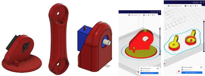
Fig.1. Design of the robotic arm

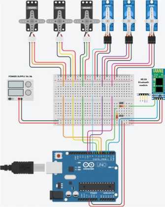
Fig.2. The control circuit of the robotic arm (a); the mobile phone application interface (b)

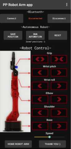
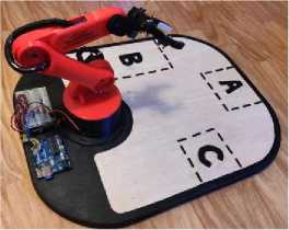
Fig.3. The complete robotic arm (a); the CAD model of the 3D Printed Robot “Thangs” (b)

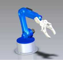
The main goal is to create the appropriate programs for the compatibility between the Android application with the Arduino and the robotic arm via Bluetooth. The application allows the movements of all axes as well as the adjustment of the speed of the servomotors. Also, the user can save arm positions to implement an automated movement (Fig. 3a). The kinematics of the model was then analyzed to test it successfully and measure its accuracy and efficiency. The 3D printed Robot, shown in digital form Figure 3b, is a small-scale desktop robot with 5 axes plus the gripper. It was designed in separate .stl files in order to be 3D printed and connected to its motors which are controlled with an Arduino board. After the joints were printed there were imported in Autodesk Fusion 360 software and the link lengths and joint offsets were measured.

The simulation software that was used is RoboDK. This software can only manage 4 axes or 6 axes robots. For that reason, a six axis table was added for the proper TCP calculation. RoboDK constitutes a newer entry compared to other commercially available software that are dedicated to robotic applications [28,29], providing a cost-effective alternative. With that measurements all the data needed for the DH parameters table were collected in Table 1.

Table 1. DH parameters

Link	Link Length (ai), mm	Twist angle (αi), deg	Joint offset (di), mm	Joint angle (θi), deg
1	a1 = 13.919	90	d1 = 97.453	(θ1)
2	a2 = 120.000	0	d2 = 0.000	(θ2)-90
3	a3 = -5.477	90	d3 = -12.700	(θ3)
4	a4 = 5.000	-90	d4 = 119.700	(θ4)
5	a5 = 9.100	90	d5 = 12.500	(θ5)
6	a6 = 0.000	0	d6 = 122.400	(θ6)+180

The required data collected for the DH table were introduced to the simulation software RoboDK using its robot configuration tool shown in Fig.4.

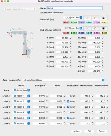
Fig.4. RoboDK’s Robot configuration tool

Robot - Export Robot Kinematics

41 paste data

Kinematics           Model

О Nominal        О Denavit Hartenberg (DH)

Accurate          Denavit Hartenberg Modified (DHM)

copy data

	a (deg)	a (mm)	8 (deg)	d (mm)
Joint 1	90.000	13.919	0.000	97.453
Joint 2	0.000	120.000	90.000	0.000
Joint 3	90.000	-5.477	0.000	-12.700
Joint 4	-90.000	5.000	0.000	119.700
Joint 5	90.000	9.100	0.000	12.500
Joint 6	0.000	0.000	180.000	122.400

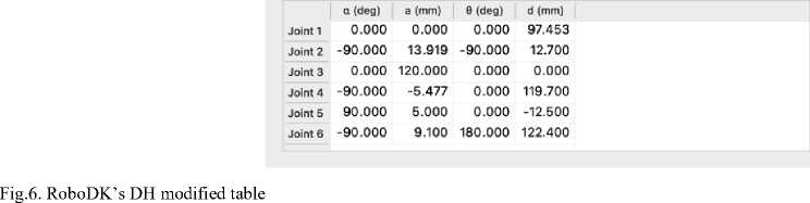
Fig.5. RoboDK’s DH table

There are some deviations from the data in Table 1 and that’s why RoboDK uses a modified version of DH Model. As shown in Fig.5 and Fig.6 each a(i) is used as a(i+1) and d2=-d3. The value a(4) of DH (a(5) of modified DH) was inserted directly to the table since there was no dedicated field for that in the configuration tool.

• •                 Robot - Export Robot Kinematics

Kinematics            Model

В paste data

Nominal           Denavit Hartenberg (DH)

Accurate О Denavit Hartenberg Modified (DHM)           copy data

For calculation of the forward kinematics the Denavit and Hartenberg matrix method were used to construct the coordinate system connected to each link in the robot’s joint chains to describe the translational and rotational relationship between adjacent links. Transformations between two consecutive joints can be written by substituting the parameters in the parameter table in their corresponding place in the matrix called “T_i ^i-1 ” (1), where:

	cos(θi)	- sin(θi) cos(αi)	sin(θi) sin(αi)	ai cos(θi)
T i i-1 =	sin(θi)	cos(θi) cos(αi)	- cos(θi) sin(αi)	ai sin(θi)	(1)
	0	sin(αi)	cos(αi)	di
	0	0	0	1

For links 1 to 6 the transformation matrixes are: A 1 is the transformation matrix T₁ ⁰ (2):

	cos(θ1)	- sin(θ1) cos(α1)	sin(θ1) sin(α1)	a1 cos(θ1)
T 10 =	sin(θ1)	cos(θ1) cos(α1)	- cos(θ1) sin(α1)	a1 sin(θ1)	(2)
	0	sin(α1)	cos(α1)	d1
	0	0	0	1

By placing the values a1=13.919, α1=90 and d1= 97.453 in the above equation, the following equation (3) which is the resultant for the transformation between the base and joint 1 is obtained:

cos(θ1)

0 sin(θ1)

1 0

sin(θ1)

-

13.919 cos(θ1)

cos(θ1) 13.919 sin(θ1)

97.453

For A 2 = T 2¹ (4):

cos(θ2)

sin(θ2) T=

- sin(θ2) cos(α2) sin(θ2) sin(α2) a2 cos(θ2) cos(θ2) cos(α2) - cos(θ2) sin(α2) a2 sin(θ2) sin(α2)           cos(α2)          d2

0   01

By placing the values a2=120, α2=0 and d2= 0 in the above equation, the following equation which is the resultant for the transformation between joint 1 and joint 2 is obtained (5):

	cos(θ2)  - sin(θ2)  0  120 cos(θ2)
T21	sin(θ2)   cos(θ2)   0  120 sin(θ2) =   0     01    0                       (5) 0   00  1

For A 3 = T 3² (6):

cos(θ3) sin(θ3) T= 30 0

- sin(θ3) cos(α3)   sin(θ3) sin(α3)   a3 cos(θ3) cos(θ3) cos(α3)   - cos(θ3) sin(α3)  a3 sin(θ3) sin(α3)            cos(α3)          d3 0   01

By placing the values a3=-5.477, α3=90 and d3=-12.7 in the above equation (7), the following equation which is the resultant for the transformation between joint 2 and joint 3 is obtained:

	cos(θ3)  0   sin(θ3)   -5.477 cos(θ3)
T32 =	sin(θ3)  0  -cos(θ3)  -5.477sin(θ3) 0     1      0           -12.7                                         (7) 00  0     1

For A 4 = T 4³ (8):

cos(θ4) 3     sin(θ4) 0

- sin(θ4) cos(α4)   sin(θ4) sin(α4)   a4 cos(θ4) cos(θ4) cos(α4)   - cos(θ4) sin(α4)  a4 sin(θ4) sin(α4)            cos(α4)          d4 0   01

By placing the values a4=-5, α4=-90 and d4=119.7 in the above equation (9), the following equation which is the resultant for the transformation between joint 3 and joint 4 is obtained:

cos(θ4) 0   - sin(θ4) 5 cos(θ4)

T 4³

sin(θ4) 0 cos(θ4) 5 sin(θ4) 0     -1      0        119.7

00  0    1

For A 5 = T 5⁴ (10):

[cos(θ5) sin(θ5)

- sin(θ5) cos(α5) cos(θ5) cos(α5) sin(α5) 0

sin(θ5) sin(α5)

- cos(θ5) sin(α5) cos(α5)

a5 cos(θ5) a5 sin(θ5) d5

]

By placing the values a5=9.1, α5=90 and d5=12.5 in the above equation (11), the following equation which is the resultant for the transformation between joint 4 and joint 5 is obtained:

cos(θ5)

_{T 5} 4 ₌

sin(θ5) 0

0 sin(θ5) 9.1 cos(θ5)

0  - cos(θ5) 9.1 sin(θ5)

1       0           12.5

00   1

The final equation is for the 6th axis. Since the robot does not have one it’s only serves to obtain the final TCP in regard of the length of the gripper/5th axis. Since there is no 6th axis it cannot rotate so the θ value will be (θ6=0) +180 = 180 degrees to compensate for the Δθ=180 that RoboDK applies to the 6th axis for the orientation of the TCP.

For A 6 = T 6⁵ (12):

[cos(θ6) sin(θ6)

- sin(θ6) cos(α6) cos(θ6) cos(α6) sin(α6) 0

sin(θ6) sin(α6)

- cos(θ6) sin(α6) cos(α6)

a6 cos(θ6) a6 sin(θ6) d6

]

By placing the values a6=0, α5=0, d5=122.4 and θ6=180 in the above equation (13), the following equation which is the resultant for the transformation between joint 5 and the final TCP is obtained:

	-1	0	0	0
T 65 =	[ 0 0	-1 0	0 1	0 122.4
	0	0	0	1

For A 123 = T 3⁰ (14):

T 30 = T 10 XT 21 XT 32 =

cos(θ1)	0	sin(θ1)	13.919 cos(θ1)		cos(θ2)	- sin(θ2)	0	120cos(θ2)		cos(θ3)	0	sin(θ3)	-5.477cos(θ3)
sin(θ1)	0	- cos(θ1)	13.919 sin(θ1)	* ·	sin(θ2)	cos(θ2)	0	120sin(θ2)	* ·	sin(θ3)	0	- cos(θ3)	-5.477 sin(θ3)	(14)
0	1	0	97.453		0	0	1	0		0	1	0	-12.7
0	0	0	1		0	0	0	1		0	0	0	1

The resultant transformation between the base and joint 3 is illustrated (15) as follows:

cos(θ1) cos(θ2 + θ3) sin(θ1) cos(θ2 + θ3) sin(θ2 + θ3) 0

sin(θ1)

-cos(θ1) 0 0

cos(θ1) sin(θ2 +θ3) cos(θ1) (120cos(θ2) + 13.919 sin(θ1) sin(θ2 +θ3) sin(θ1) (120cos(θ2) + 13.919

- cos(θ2 + θ3) 0

- 5.477 cos(θ2 + θ3)) - 12.7sin(θ1)

-

5.477 cos(θ2 + θ3)) + 12.7 cos(θ1)

120sin(θ2) - 5.477 sin(θ2 +θ3) + 97.453 1

]

For A 456 = T 6³

(16):

T63 = Т43хТ54хТ65 = cos(θ4) sin(θ4) 0 0

-1 0

- sin(θ4) cos(θ4) 0

5 cos(θ4) cos(θ5)

5 sin(θ4)

119.7

·

sin(θ5)

1 0

sin(θ5)

- cos(θ5)

9.1 cos(θ5)

9.1 sin(θ5)

12.5

·

-1 0 0 0

-1 0 0

1 0

122.4

The resultant transformation (17) between joint 4 and the final TCP is illustrated as follows:

T 6³ = [

-cos(θ4) cos(θ5)

-sin(θ4) cos(θ5) sin(θ5) 0

sin(θ4)

-cos(θ4) 0 0

cos(θ4) sin(θ5) cos(θ4) (9.1 cos(θ5) + 122.4 sin(θ5) + 5) - 12.5 sin(θ4) sin(θ4) sin(θ5) sin(θ4) (122.4 sin(θ5) + 9.1 cos(θ5) + 5) + 12.5 cos(θ4)

cos(θ5) 0

122.4cos(θ5) - 9.1 sin(θ5) + 119.7 1

]

The final transformation matrix

kinematics equations of the robot is (18):

for the tool coordinates along a serial robot consisting of n

links

from the

T 6⁰ = ^∏ iⁿ=1 T i^i-1

Where T_i ^i-1 is the homogeneous transformation matrix of the link i related to link i-1. For A 123456 = T₆ ⁰ , for simplicity (19-24):

A= cos(θ1) (120cos(θ2) + 13.919 - 5.477cos(θ2 + θ3)) - 12.7sin(θ1)

B = sin(01) (120 cos(02) + 13.919 - 5.477 cos(02 + 03)) - 12.7 cos(01)

C = 120 sin(θ2) - 5.477 sin(θ2 + θ3) + 97.453

D = cos(θ4) (9.1cos(θ5) + 122.4sin(θ5) +5) - 12.5sin(θ4)

E =sin(θ4) (122.4sin(θ5) +9.1cos(θ5) +5) + 12.5 cos(θ4)

F = 122.4cos(θ5) -9.1sin(θ5) + 119.7

T 60 = T₁ ⁰ xT₂ ¹ xT₃ ² xT₄ ³ xT_s ⁴ xT 6^; = T₃ ⁰ xT₆ ³

T 6 ⁰ = [

cos(θ1) cos(θ2 + θ3)	sin(θ1)	cos(θ1) sin(θ2 + θ3)	A   -cos(θ4) cos(θ5) B   -sin(θ4) cos(θ5) C         sin(θ5)	sin(θ4)	cos(θ4) sin(θ5)
sin(θ1) cos(θ2 + θ3)	-cos(θ1)	sin(θ1) sin(θ2 + θ3)		-cos(θ4)	sin(θ4) sin(θ5)
sin(θ2 + θ3) 0	0 0	- cos(θ2 + θ3) 0		0 0	cos(θ5) 0

DF1E]

The result is a 4x4 matrix (25-27) that gives the information about the orientation matrix and position.

r11 r12 T60 = r21 r22 r31 r32 0 0 r13   Px r23  Py r33   Pz

In which (28-39):

r11 = sin(05) cos(01) sin(02 + 03) —cos(04) cos(05) cos(01) cos(02 + 03) — sin(04) cos(05) sin(01)(28)

r12 = sin(04) cos(01) cos(02 + 03) — cos(04) sin(01)(29)

r13 = cos(04) sin(05) cos(01) cos(02 + 03) + sin(04) sin(05) sin(01) + cos(05) cos(01) sin(02 + 03)(30)

r21 = sin(04) cos(05) cos(01) + sin(05) sin(01) sin(02 + 03) — cos(04) cos(05) sin(01) cos(02 + 03)(31)

r22 = sin(04) sin(01) cos(02 + 03) + cos(04) cos(01)

r23 = cos(04) sin(05) sin(01) cos(02 + 03) — sin(04) sin(05) cos(01) + cos(05) sin(01) sin(02 + 03)(33)

r31 = —cos(04) cos(05) sin(02 + 03) — sin(05) cos(02 + 03)(34)

r32 = sin(04) sin(02 + 03)(35)

r33 = cos(04) sin(05) sin(02 + 03) — cos(05) cos(02 + 03)(36)

Px = Л + D cos(01) cos(02 + 03) + F cos(01) sin(02 + 03) + F sin(01)(37)

Py = В + D sin(01) cos(02 + 03) + F sin(01) sin(02 + 03) — F cos(01)(38)

Pz = C + D sin(02 + 03) — F cos(02 + 03)(39)

The lowest row in the resulting 4x4 transformation matrix is considered as the ineffective row. The top left 3x3 matrix is the rotation matrix, and the 3x1 matrix from top to bottom in the far right column is the translation matrix.

Which means the T j transformation matrix can be represented in terms of R j and P₆ ⁰ illustrated as follows (40-41):

' rii

Т б⁰ =

r21

^r31 0

r12 r22 r32

r13   Px r23  Py

Г 33    P z

0    1J

Т б⁰

R 6 0

P O ]

The translation matrix from the base coordinate system of the robot to the tip of the robot (42):

ЧП

Accordingly, the rotation matrix from the base coordinate system of the robot to the tip of the robot (43):

r11   r12

R 6 = |r 21   r 22

r31   r32

The unit vector shows the direction of the X, Y and/or Z-axis at the robot tip according to the base coordinate system. However, the expectation is to express all of these in angular form rather than vectorial. Below find how to express tip rotation in XYZ Tait-Bryan Euler angles corresponding to the order yaw-pitch-roll (44-46):

Yaw angle: C= tan-1(r21/r11) = atan2(r21, r11)

Pitch angle: B = —sin-1(r31) = —asin(r31)

Roll angle: A = tan-1^^) = atan2(r32, Гзз)(46)

The yaw and roll angles will always be in the range -π to +π (-180° to +180°). The pitch angle will be between -π/2 and +π/2 (-90° to +90°). In case the Pitch angle B equal +/- 90° (gimbal lock) then:

If Pitch angle B equal -90° (47):

A + C = atan2(—r12, —r13)(47)

If Pitch angle B equal +90° (48):

A — C = atan2(r12, r13)(48)

In practice one of A or C is set to 0 and the equations is solved for the other. In this model A will be considered as 0 and the equations will be solved for the C. This concludes the forward kinematics calculation.

4.    Experimental Results

To carry out the experimental process in order to validate the digital twin, the robot was moved to several axis positions, and final positions of the TCP regarding its base were measured and compared to the digitals twin’s results, as well as the results from the equations (Fig. 7).

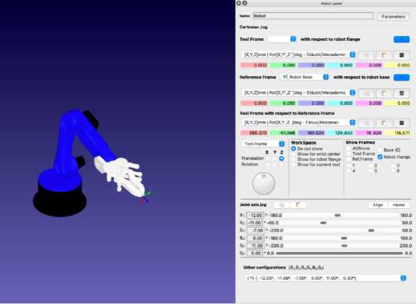
Fig.7. Taking results from digital twin in RoboDK

In the measurements below, only the final position of the end effector is included without checking the orientation. So, the comparison table that follows (Table 2) uses the right kinematic model to calculate based on the set of joint angles the final position of the end effector and the relative deviations are presented.

Table 2. Result table in mm and degrees

Axes Angles θ i	Actual Robot Values(mm) - [x,y,z]	RoboDK Values (mm) -[x,y,z]	Values from Equations (mm) - [x,y,z]	Deviation (mm) [x,y,z]
[0,0,0,0,0]	[250, 0, 221]	[256, 0, 226]	[256, 0, 226]	[6, 0, 5]
[36,23,-36,19,12]	[170, 110, 185]	[172, 110, 181]	[172, 110, 181]	[2, 0, 4]
[-28,-7,-9,-23,-14]	[217, -120, 137]	[223, -124, 135]	[223, -124, 135]	[6, 4, 2]
[14,12,-17,17,11]	[220, 46, 215]	[224, 45, 220]	[224, 45, 220]	[4, 1, 5]
[-12,-11,-7,9,11]	[270, -60, 173]	[265, -61, 169]	[265, -61, 169]	[5, 1, 4]
[90,-45,60,-60,45]	[-93, 281, 285]	[-91, 277, 286]	[-91, 277, 286]	[2, 4, 1]
[80,-40,55,-50,40]	[-25, 282, 309]	[-25, 284, 303]	[-25, 284, 303]	[0, 2, 6]
[70,-35,50,-40,35]	[40, 271, 318]	[40, 275, 315]	[40, 275, 315]	[0, 4, 3]
[60,-30,45,-30,30]	[103, 256, 322]	[101, 253, 321]	[101, 253, 321]	[2, 3, 1]
[50,-25,40,-20,25]	[154, 217, 325]	[154, 220, 322]	[154, 220, 322]	[0, 3, 3]
[40,-20,35,-10,20]	[197, 182, 321]	[196, 178, 319]	[196, 178, 319]	[1, 4, 2]
[30,-15,30,0,15]	[228, 131, 317]	[226, 131, 313]	[226, 131, 313]	[2, 0, 4]
[20,-10,25,10,10]	[249, 85, 302]	[244, 83, 303]	[244, 83, 303]	[5, 2, 1]
[10,-5,20,20,5]	[254, 37, 292]	[251, 36, 292]	[251, 36, 292]	[3, 1, 0]
[0,0,15,30,0]	[248, -5, 282]	[247, -5, 280]	[247, -5, 280]	[1, 0, 2]
[-10,5,10,40,-5]	[234, -40, 268]	[237, -40, 269]	[237, -40, 269]	[3, 0, 1]
[-20,10,5,50,-10]	[222, -71, 261]	[221, -69, 259]	[221, -69, 259]	[1, 2, 2]
[-30,15,0,60,-15]	[205, -93, 254]	[202, -91, 251]	[202, -91, 251]	[3, 2, 3]
[-40,20,-5,70,-20]	[187, -109, 246]	[183, -107, 245]	[183, -107, 245]	[2, 2, 1]
[-50,25,-10,80,-25]	[166, -117, 246]	[163, -119, 243]	[163, -119, 243]	[3, 2, 3]
[-60,30,-15,90,-30]	[142, -125, 244]	[143, -126, 243]	[143, -126, 243]	[1, 1, 1]
[-70,35,-20,100,-35]	[126, -131, 248]	[123, -130, 246]	[123, -130, 246]	[3, 1, 2]
[-80,40,-25,110,-40]	[104, -132, 252]	[104, -131, 251]	[104, -131, 251]	[0, 1, 1]
[-90,45,-30,120,-45]	[86, -131, 255]	[84, -129, 257]	[84, -129, 257]	[2, 2, 2]

The deviation values in the end effector positions in the X-axis range from 0% to 3.3%, in the Y-axis from 0% -3.2% and in the Z-axis from 0% - 2.4%. Further analysis of the discrepancies between the computational model and the physical one, is presented in Fig. 8 below.

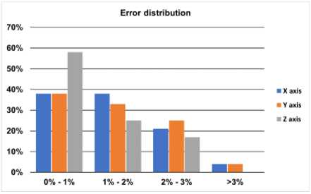
Fig.8. The error distribution for the three axes

On the X-axis 38% of the measurements have an error between 0% and 1%, 38% between 1% and 2%, 21% between 2% and 3%, and only 4% above 3%. Correspondingly on the Y axis the percentages are similar with 38%, 33%, 25% and 4% in the respective categories while on the Z axis with 58%, 25%, 17% and 0%.

5.    Conclusions

Sumarizing, this study introduces a cost-effective approach to constructing a digital robotic platform, leveraging CAD models of a 5DoF robotic arm and its physical counterpart. The design phase utilized a widely available CAD system, and the robot was assembled using 3D-printed components, demonstrating a low-cost and efficient solution. The incorporation of an Arduino UNO microcontroller further enhanced the affordability and practicality of the system. The RoboDK software played a crucial role in seamlessly converting the CAD model into a fully controllable simulation, faithfully representing the kinematics of the physical model.

The experimental validation involved a comprehensive analysis of the end-effector positioning. By comparing the final positions of the TCP in multiple axis positions, the study revealed deviations between the physical robot and the digital twin. In the X-axis, 38% of measurements exhibited errors between 0% and 1%, 38% between 1% and 2%, 21% between 2% and 3%, and only 4% exceeded 3%. Similarly, on the Y-axis, the distribution was 38%, 33%, 25%, and 4%, and on the Z-axis, 58%, 25%, 17%, and 0%.

While the majority of measurements demonstrated high accuracy, it is essential to acknowledge and address the observed deviations. The discrepancies, though minimal, provide valuable insights for further refinement and optimization of the digital twin. This study underscores the potential of the proposed methodology and highlights the need for ongoing research to enhance the fidelity of digital twins in replicating real-world robotic systems. In light of these findings, the conclusion emphasizes the practicality and efficacy of the developed digital platform, setting the stage for future advancements in the realm of robotic simulations and digital twins.