Data Visualization and its Proof by Compactness Criterion of Objects of Classes

Published Online August 2017 in MECS

The visualization is a powerful tool for searching hidden regularities at implementations of data mining techniques. In most well-known visualization techniques applied a linear mapping of the original space into one, two and three-dimensional space. The main goal pursued by researchers consists of analyzing the relationship between objects. As a rule, such an analysis makes it possible to detect hidden patterns in the data that represent the new knowledge in one or another subject area.

One of the causes of using visualization methods in data mining is to find logical patterns. The complexity of this searching is related to the decision of the NP -complete problem. A classic example of using the visualization in data mining is the method of the local geometry [1]. Searching logical regularities by using this method required an active participation of researchers in the process. New knowledge obtained from the database by applying statistical methods to them on the results of the visualization.

In [1] it was concluded that for the research of structure of the set of logical rules most suitable methods are multidimensional scaling and hierarchical agglomerative procedures of cluster analysis. These methods allow to get the visual representation of the geometric structure of the aggregate logical regularities and their results are complemented each other.

In this paper we offer to apply a nonlinear mapping the description of objects on numerical axis with the rules of hierarchical agglomerative grouping. It is proved the truth of the statement that latent features which obtained as a result of mapping express the compactness of class objects better than the initial space of the raw features. The latent features which formed as a result of grouping, obtained ordered by the degree of informativeness.

In this paper considered the criteria for the estimation of different visualization methods. Most often visualization is interpreted as a problem of reducing the dimension of the space by the transition to the new features in the description of objects. There are a lot of criterions which optimizations [2] aim to preserve the original and the new space structure through the distance between objects. The estimation of local compactness is oriented on checking the similarity of class objects (including the visualisation) [3].

In this paper presented the basis of using the criterion for analyzing the structure of relatedness of objects through the so-called shell (a subset of the boundary objects) classes. As the shell [4] used a subset of the boundary objects of classes by a given metric. The value of the offering criterion determines the degree of compactness of classes in [0,1].

The number of features plays a significant role in structured datasets. We can apply the standard algorithms and methods without difficulty to analyze the data if the size of feature space rather small, otherwise there may be a major problem, known as “curse of dimensionality”, that reduces the classification accuracy, increases the classification model complexity and increases the computational time, thus the need for Feature Selection (FS) [5] [6]. In [7] authors offered the feature selection approaches, which are capable of minimizing the number of selected features without reducing the classification accuracy of all features .

Searching informative features set usually be used to estimate the classification accuracy of the algorithms. In [8] a genetic algorithm (GA)-based features selection to improve the accuracy of medical data classification is proposed. In [9] developed a novel feature selection technique based on the Partial Least Squares (PLS). PLS aims to obtain a low dimensional approximation of a matrix that is ‘as close as possible’ to a given vector. The main purpose of the proposed method is to select the significant feature subset which gives the higher classification accuracy with the different classifiers.

In the form of the computational experiment on the test example proved that the degree of compactness in nonlinear data mapping higher than the method of PCA.

This paper is organized as follows. Section I provides an overview of the most significant related work and the structure of the paper. Section II describes the problem statement, research purpose, requirements and theoretical basis. In section III discussed some another method to verify the obtained result and an algorithm based on this method. Section IV presents the computational experiment. Section V concludes the paper.

• II.    Problem Statement

The two class recognition problem is considered in a standard formulation. Objects of the sample E_o = { S ,..., S_m } belong to one of the classes K_x or K ( E _o = K U K ) and each object is described using n different - type features X(n) = (x_p ^ ,x_M) , a set of permissible values § of which is measured on the interval scales, and n - § is measured on the nominal scale. It is considered that in X ( n ) given a linear and nonlinear mapping of objects descriptions on numerical axis. The nonlinear mapping is implemented by sequential partitioning a set of X ( n ) according to the rule of hierarchical agglomerative groupings in X_x ( k_x ) ,..., X_T ( k ) , t >  1, k + ...+ k_T <  n disjoint subsets. Each subset of X_x ( k_t ) , t = 1, ^ , г is mapped on the numerical axis and is considered as a new latent feature in the description of the objects. It is required:

• •    generate a new space of latent features for mapping object descriptions to the plane with the algorithms of the linear and nonlinear methods;

• •    give a numerical estimation of placement structure of the class object descriptions in space which based on defined measure proximities.

To implement linear and nonlinear methods used proof of the truth of the compactness hypothesis in the form of a computational experiment. The proof is based on the following criteria which proposed partitioning the values of feature into intervals.

Let us assume that on E defined the ordering of objects by any of its property q , which given (initial values of a quantitative attribute), or defined by an algorithmic way.

q ( S i ), q ( S i ), ... , q ( S i ). (1)

The ordered set of values (1) is divided into two disjoint intervals [ c , c ] , ( c , c ] , each of them is considered as the gradation of the nominal feature. The criterion for determining the boundaries of c is based on checking the hypothesis (statement) that each of the two intervals contains the values of a quantitative value of only one class objects.

Let u1, u2  - the number of values (1) by some quantitative (the initial or latent) feature of class K, i = 1,2 accordingly in the intervals [cQ, cx ] , (cx, c2 ] , IK. I > 1, v - the sequential number of the ordered element in ascending order (1) in E , which defines the boundaries           of           intervals           as c0 = q(S ), c = q(S.), c2 = q(St ) . The criterion

22        22

ZZ u ( u - 1 ) ZZ u (I ^K 3 - i l- uD ^d = 1 i = 1-------------------- ^d = 1 i = 1------------------------------

Z i k ki k i- 1)         21 ^к >' 21

• V i = 1                   7 V                             7

^ max c1 < c 2 < c 3

allows to calculate the optimal value of the boundaries between intervals [ c , c ] , ( c , c ] . The expression on the left-hand brackets (2) is the intraclass similarity and in the right - interclass difference.

For the convenience of exposition, we denote the set of indexes of quantitative features through I , and nominal features by J . We consider the calculation of the weights and contribution of the nominal features grades which are used in both linear and nonlinear methods.

Let us denote by p the number of gradation of the feature r e J , g⁽_dr - a number of values of the t -th ( 1 <  t <  p ) gradation of the r -th feature in the description of objects of the class K , l - a number of gradation of the r -th feature in K . The difference over the r -th feature between the classes K and K is determined as a value

ZLgrg ‘^

X _r = 1 - 2=—---

The degree of uniformity (intraclass similarity measure) в gradation values of the r -th feature by classes of K , K is calculated according to the formulas:

D, 4 dr

f(| K d\ - l dr +1 )(| K d |- l dr ) , p > 2,

Pr = 1

p

У gtr (gtr - 1) + g2r (gtr -1) t=1

0,

D, + D-^ = 0.

With (3), (4) the weight of nominal feature r e J is determined as

V r = ^ r P r .

It is easy to verify that the set of weight values of nominal and quantitative features, calculated by (2) and (5) belong to the interval [ 0,1 ] .

It is obvious that a set of numbers identifying as p gradation of the nominal feature, always possible one-to-one mapping into the set { 1,..., p } . Taking into account such a mapping for the object S = ( x ,..., x _n) contribution x = j , i e J , j e { 1,..., p } feature in generalized estimation is defined by

descriptions of objects with features in X ( n ) using functional R , R . In E defined division into two disjoint subsets E ¹, E ² of the representatives of K , K . In E ¹, E ² calculated the optimal values of the functional R , R according to (8), which are used for mapping objects of E in two numerical scales. It is proved the equivalence of these two scales by (2) in [10].

In algorithms of nonlinear mapping to calculate the values of defined set of features in the description of objects used hierarchical agglomerative grouping rules [11]. For identifying the features as an initial so an obtained by calculating the generalized estimation on the p-th step (0 < p < n) of grouping will use {xp} ,   , where |I| + |J| = n at p = 0 . The extremum of the criterion (2) is used as a weight wp (0 < wp < 1) of the feature xp . At wp = 1 the values of the feature xp of objects in classes K, K do not intersect between themselves. The value of generalized estimation bp (latent feature’s) of the object Sr = (ap ,..., ap„_p) , Sr e E0 by pair of (xp, xp ) , 1 < p < nPi, j e IPi * j is calculated as

A ^(a p ) ⁺ A j ^(a p ), iJ ^{e J}

I a p - c j ^p

A (ap ) + t,wp —----- i ri        j j       jp       jp c-

, i e J , j e I

—

A i ^{( j} ) =

^p rij

n ij

I a^p - c p _twpri    2

2 c ip - c^p

p      jp arj   c2

jp       jp cc

where a1, a2 -are the numbers of the values of j th ij ij gradation by i -th feature accordingly in classes K and K , v - is a weight of the i -th feature, calculating by (5). In different – type features space generalized estimation for each object Sa e E0 , Sa =(xa 1,...,xan) will be calculated as

R ( ^Sa )   У wt ( x ai - c i ) / ( c 2 - c 0 )⁺У A ( x a, )    ⁽⁷⁾

iel                                               ieJ where wz, i e I , and the boundary of the interval ci is calculated as optimal value of the feature x e X(n) by (2) on Eo , and the vector   T = ( tx,..., tn), t e{-1,1} is defined from the condition

min ^{R ( S} a ^)- max ^{R ( S} a H max.         ⁽⁸⁾

S a ^{e K} 1                S a ^{e K} 2                    E 0

In presenting objects by linear method on the plane will select two numerical scales for mapping to them

⁺ ( 1 ^- n ij ) t ij w ip

I a^pa^p -cij ri rj       2

I    ijpp _ ijyp

2 c 3 ^c 1

, i , j e I

where A i (a p .), A j (a p .)are calculated by (6), w f ,w p ,w ^p – are the weights of the features, which defined by (2) accordingly by the set of features values x^p , x^p and their

multiplication        x^px^p

the       values

t, , tj , t_y e { -1,1 } , n e [ 0,1 ] are selected by extremum of

the functional

ф ( p , i , ^j ) =

min b p - max b p

Sr e K 1 rj    Sr e K2  rj max bp - min bp

S r e E 0   rj   S r e E ₀   ^r j

max .

The value (10) is interpreted as an offset between objects of the classes K and K . A detailed description of the algorithm for selecting the latent features by (9) and (10) can be found in [11].

The latent features calculated by the (9) form a new space for the object descriptions in recognition algorithms. Analytical representation of nonlinear transformations

proposed in [12], makes it possible to use the results of the described algorithm as a decision rule for recognition.

In nonlinear methods opposed to the linear, we cannot say about the equivalence of two numerical scales for the display of objects descriptions. It is proposed to use the values of the first two latent features for visualization because of they have the highest indexes of separability of objects projection by criterion (2). The proof of the statement is based on the criterion of compactness of class objects.

• III.    Cluster Analysis and Compactness of Class Objects

The main purpose of dividing the class objects into disjoint groups is the calculation and analyzing compactness values of objects of classes and sample as a whole by the result of visualization. The compactness is offered to calculate by the results of grouping algorithm [13] of representatives of classes according to their relatedness through the defined subset of the boundary objects. As a distance p (x,y) between the objects in E_o is used a metric of Juravlyev. The metric of Juravlyev allows analyzing the structure of class objects considering the features variety.

Let we denote through L(Eo, p) - the subset of boundary objects of classes, which is defined in E by the metric p(x,y) . The objects St, S e K, t = 1,2 are considered to be related to each other (Sz. ^ S.) , if {S e L(E0, p) | p(S, S) < r and p(S, Sy) < r.} ^ 0 , where r(r)- is the distance from S(S) to the nearest object in K3t by the metric p(x, y).

The set   Gv = {S„ ,...,Sv=}, c > 2, G^ c K,,v < K presents the area (group) with related objects in class K , if for any   Sv ,Sv eG there is a way

S, ^ Sv ^... ^ S. . Object S. e K ,t = 1,2 belong to vi     vk          vj          it the group with single element and is considered not related, if there is no way Si ^ Sj for any object Si ^ Sj and Sj e Kt. It is required to define the minimum number of disjoint groups of related and unrelated objects for each class Kt, t = 1,2.

To define the minimum number of groups of related and unrelated class objects we use L (E_o, p ) - the subset of the boundary objects (shell) of classes by metric Juravlyev p and it allows us to describe the objects in the new space of binary features.

To separate the shell (boundary objects) of the class for each object S e K_t , t = 1,2 would built an ordered sequence by p (x,y) as

^S , 1 ^,...^{, S} m _ _ , S = ^.               (11)

Let S. e K__t is the nearest to S_t object from (11) not including in class K . Let us denote through O (S ) the neighborhood of S_t , with radius r = p (S., S^ ) and centered on S , including all of the objects for which p (S_/,S) < r, T = 1,..., в -1. In O (S i ) there is always nonempty subset of objects

A = {S . e OS)| p SS) = _smin ^ S , , S)}. (12)

By (12) the belonging of objects to the shell of classes m is defined as L(Eo, p) = |J Az.

г = 1

The set of shell objects in K nL(Eo,p) is denoted as L (Eo,p) = {S1,...,Sn}, n > 1. The value n = 1 unambiguously determines including all of the objects of classes into one area. When n > 2 we transform the description of each object S eKt to S = (y^.^y^) , where y j =

/1, p (S _z ,S ^j ) <  r, <0, p (S z ,S ^j ) >  r.

Let by (13) the description of objects of class K is obtained in new (binary) feature space, Q = K,6 - number of disjoint groups of objects, and S^ л S^ e Kt. The step by step execution of the algorithm of partitioning the objects of K into disjoint groups G,...,G is given as follows:

Step 1: 6 = 0;

Step 2: Separate the object S e Q , 6 = 6 + 1, Z = S , G 6 = 0 ;

Step 3: Perform the selection S e Q and S л Z = true, Q = Q \ S ,      G₆ = G₆ u S ,      Z = Z v S    until

{S eQ | S л Z = true } ^0 ;

Step 4: If Q ^ 0 , then go to 2;

Step 5: End.

To analyze the results of visualization proposed to use the structural characteristic as an estimation of the compactness of classes

1Ё m 2

6 z = ^=L2_ m

where p - is the number of groups in Kz, z' = 1,2 , m. = |K. I, mt]. - is the number of objects in the j -th group of the class K . The average estimation of compactness on the training sample is calculated using the formula

^ тД F(Eo, p) =  ----- m

where m - is the number of sample objects.

• IV.    Computational Experiment

The computational experiment was conducted with data of Echocardiogram [15]. In reality, the sample consists of 132 objects, but in this experiment, we did not consider the case of missing values in data. Therefore, all objects which have missing values are removed. So the sample consists of 108 objects, each object is described by 9 quantitative and 2 nominal features. The sample contained 74 representatives of the class K (patient was either dead after 1 year or had been followed for less than 1 year) and 34 of the class K (patient was alive at 1 year).

The methods of visualization were considered over the three features spaces.

• -    original (11 features);

• -    expanded (14 features);

• -    reduced (10 features).

An expanded space from the original different in that each gradation of nominal feature considered (by the values {0,1}) as a separate quantitative feature. In the reduced space all nominal features (in our case the two nominal features) are presented a quantitative one using the linear mapping according to (7). The dimension of the space of the latent feature, which obtained by the nonlinear method, taking into account the abovementioned three ways of describing the objects given in table 1.

Table 1.The dimension of space of the latent features

№	The space	The dimension (Values of weights of the features by (2))
1	Original	3 (0.748106, 0.452188, 0.324245)
2	Expanded	4 (0.787037, 0.517507, 0.382487, 0.335042)
3	Reduced	3 (0.748106, 0.452188, 0.324081)

The visual presentation of objects, obtained by linear [10] and nonlinear [11] methods in original feature space is given in figure 1 and figure 2. As a result of the nonlinear method (see table 1) in presentation used the first two latent features. The objects of the class K marked with “x” symbol, K₂ - “o”.

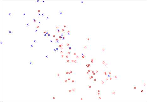
Fig.1. The visualization objects by linear method

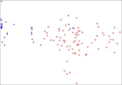
Fig.2. Visualization of objects by nonlinear method

From the image in figures, it is clear that objects of classes K and K better divided among themselves by using the nonlinear (Fig. 2) than the linear (Fig. 1) method.

Finding the groups is implemented through calculation the connectivity of objects. To demonstrate the connectivity of any two objects used a line which connects the two objects. The number of lines going out from an object means how many objects are connected to this object. And a group is the set of connected objects.

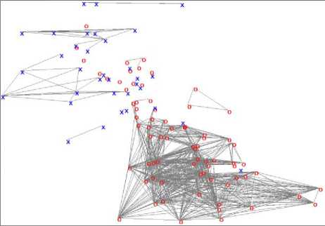
Fig.3. Grouping the objects according to the results of visualization by linear method

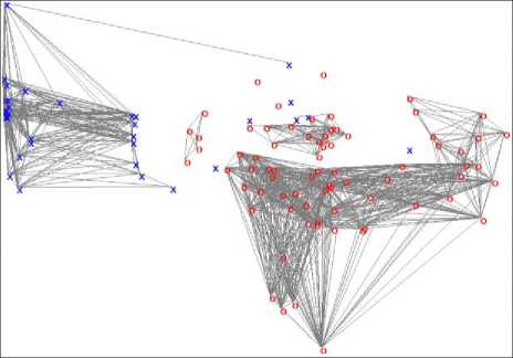
Fig.4. Grouping the objects according to the results of visualization by nonlinear method

As shown in figures 3, 4 the number of groups and its structure strongly influences when calculating the compactness. It is clear from the figure 4, that each class has equal number of groups, but the compactness are different: F(K_P p) = 0.800949 and F(K₂, p ) = 0.636678 (see table 5).

For comparative analysis, we consider the compactness of classes (14) and sample in whole (15) from the table 2, and mapping the objects by the nonlinear method in table 3. In brackets indicates the number of groups of objects and the dimension (see table 1) of the space of latent features.

Table 2. The compactness of the objects of classes (14) and sample as a whole (15)

The space	The compactness (number of groups) by
	K 1	K 2	E 0
Original	0.491234 (3)	0.833910 (4)	0.599113 (7)
Expanded	0.448867 (4)	0.833910 (4)	0.570084 (8)
Reduced	0.921110 (4)	0.782006 (5)	0.877318 (9)

Table 3. The compactness of the objects of classes (14) and sample as a whole (15) by using the results of nonlinear method

The space (the number of latent features)	The compactness (number of groups) by
	K 1	K 2	E 0
Original (3)	0.973338 (2)	0.737024 (4)	0.898943 (6)
Expanded (4)	0.800219 (4)	0.304498 (14)	0.644158 (18)
Reduced (3)	0.947041 (3)	0.782006 (5)	0.895086 (8)

It is clear from the table 2 and 3 that relatively low value of compactness is obtained when using values of features of the expanded space as a data.

The compactness indexes on the results of visualization of linear and nonlinear methods are given accordingly in table 4 and table 5. It have been used the first two latent features during the calculation by the results of nonlinear methods.

Table 4.The compactness by results of visualization using linear method

The space	The compactness (number of the groups) by
	K 1	K 2	E 0
Original	0.598612 (14)	0.252595 (13)	0.489680 (27)
Expanded	0.323228 (11)	0.233564 (13)	0.295000 (24)
Reduced	0.686267 (8)	0.297577 (7)	0.563902 (15)

Table 5. The compactness by results of visualization using nonlinear method

The space	The compactness (number of the groups) by
	K 1	K 2	E 0
Original	0.800949 (6)	0.636678 (6)	0.749234 (12)
Expanded	0.133674 (17)	0.429065 (13)	0.226667 (30)
Reduced	0.846603 (5)	0.647058 (5)	0.783783 (10)

To visualize by the linear method used mapping the objects by values of all features of the original space into two equivalent scales [10]. And the indexes of compactness (see table 4) were worse than using the nonlinear method (see table 5). The confirmation of this fact may be seen when comparing the images in figure 1 and figure 2.

To compare the results of linear and nonlinear methods with one of the well-known method as PCA, we used SPSS Statistics (Statistical Package for the Social Sciences) software package. There is the result of PCA method adequately consideration all factors (which eigenvalues greater than 1 [14]) and the first two factors in table 6.

Table 6. The compactness of the objects of classes (14) and sample as a whole (15) using PCA

The space	The compactness (number of groups) by
	K 1	K 2	E 0
By all components	0.448502 (12)	0.243944 (11)	0.384104 (23)
By the first two components	0.600073 (8)	0.411764 (9)	0.540790 (17)

From the tables 5 and 6, we can see that using nonlinear method gives much better compactness by classes so and by sample as a whole than PCA method (see first row of the table 5 and the second row of the table 6).

The visual presentation of objects by PCA method using the first two factor (based on the first two eigenvalues) as a latent feature is presented in figure 5 and groups of objects are in figure 6.

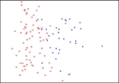
Fig.5. Visualization of objects by PCA

From the figure 5, we can see that when we use PCA method for visualization a lot of objects of different classes are intersect each other than using nonlinear method (see figure 2)

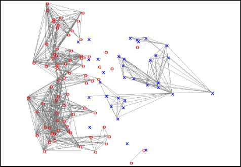
Fig.6. Grouping the objects according to the results of visualization by PCA

• V. Conclusions

It is proved the effect of using the nonlinear method to form the space of latent features in the description of objects in pattern recognition problems. The indexes of effect serve an estimation of objects of the classes and the sample as a whole. The results of visualization may be used when searching the hidden regularities in databases.