Development and implementation of machine learning models for inventory forecasting in technology companies

Вестник Российского нового университета

Серия «Сложные системы: модели, анализ и управление». 2026. № 1

On AI-based decision support systems for inventory management is underlined by a set of converging elements that have positioned inventory optimization as a strategic priority and not an operational problem [3]. Firstly, inventory represents a significant capital expense for organizations in any industry, with the global inventory management software market expected to reach $3.2 billion by 2026, underscoring the significant economic relevance of the domain. Second, the pandemic of COVID-19 has disclosed significant vulnerabilities of global supply chains, ruthlessly illuminating the consequences of overstocking (wastage and obsolescence) and poor inventory levels (stockouts and forgone sales), thereby more forcefully emphasizing the need for more resilient and responsive inventory control practices [4]. Third, the resultant exponential rise in data availability–through enterprise resource planning systems, Internet of Things sensors, and digital supply chain platforms–has created unprecedented opportunities for sophisticated analytics previously not possible, but most organizations are struggling to leverage this data abundance to derive meaningful inventory insights. Fourth, despite the advances in machine learning and AI, research indicates that almost 79% of companies still significantly rely on spreadsheets or basic software for inventory choice, indicating a colossal gap between technological potential and actual adoption [5]. Fifth, increasing pressure for sustainability across business activities means enhanced precise inventory management to reduce waste, reduce carbon emissions, and improve circular economic practices. Sixth, inventory positioning has become more difficult with e-commerce and omnichannel retailing and decreased the desirable level of inventory imbalance, as the customer expects instant availability of the product through every channel [6]. Finally, academic research has tended to focus on individual building blocks of inventory management–demand forecasting, optimization models, risk analysis, or pricing policy–without much regard for overall frameworks that deal with the interdependencies between these components. This research answers such fragmentation by an overarching methodological approach that leverages artificial intelligence for the entire lifecycle of inventory management, particularly relevant to the present period of dynamic business where operational efficiency and supply chain resilience have become central drivers of competence. General issues of machine learning and predictive modeling have been extensively examined in the works of T. MITCHELL, I. GOODFELLOW, A. NG, and Y. BENGIO. Significant contributions to feature selection techniques, particularly recursive feature elimination and ensemble learning approaches, have been made by J. FRIEDMAN, L. BREIMAN, S. SHALEV-SHWARTZ, and A. STREHL. In the context of inventory management and demand forecasting, the studies of P. W. C. PRASTACOS, C. CHIEN, S. V. CHOPRA, and M. A. FISHER have highlighted the potential of machine learning models to optimize supply chains and predict sales dynamics. Furthermore, the integration of intelligent technologies into inventory optimization strategies has been investigated by L.R. MARTIN and E.G. DEMEYERS [7].

• 2.    Methodology

• 2.1.    Conceptual Design of the Decision Support System

The methodological framework of the AI-powered decision support system for inventory management establishes the structural foundation upon which the four analytics blocks are integrated [8]. This structure details the conceptual architecture, integration framework, and data processing pipeline that enables efficient interaction between the demand forecasting, inventory optimization, supply chain risk analysis, and dynamic pricing blocks. The architecture

Development and implementation of machine learning models for inventory forecasting in technology companies is designed to facilitate both real-time decision support as well as strategic planning in an integrated system where component autonomy is facilitated while coordinating their tasks [9].

The methodological choices adopted in this study are guided by a comparative assessment of alternative approaches commonly applied in inventory forecasting and control. Classical statistical models and rule-based inventory policies are widely used due to their simplicity and interpretability; however, they typically rely on strong assumptions regarding demand stationarity, linearity, and independence, which are rarely satisfied in dynamic and data-intensive environments characteristic of technology companies.

Machine learning models, in contrast, offer greater flexibility in capturing non-linear relationships and complex feature interactions but are often applied in isolation to specific subproblems, such as demand forecasting or pricing optimization. The proposed methodology addresses this limitation by integrating multiple machine learning components within a unified decision support framework, allowing predictive outputs from one module to systematically inform and constrain the behavior of others. This design choice distinguishes the proposed approach from single-model or single-task methodologies and enables consistent decisionmaking across the inventory management lifecycle.

From a generalizability perspective, the methodology emphasizes structural robustness rather than reliance on a particular dataset or algorithm. The use of modular architecture, standardized data interfaces, and time-aware validation strategies allows individual components to be retrained or replaced without altering the overall system logic. Moreover, validation procedures based on expanding time windows, scenario-based simulations, and stress testing under demand and supply uncertainty are incorporated at the methodological level to assess model stability beyond average-case performance.

As a result, the proposed methodology is not tied to a specific industry configuration or demand distribution but provides a transferable framework that can be adapted to different operational contexts through feature engineering, parameter tuning, and domain-specific data integration.

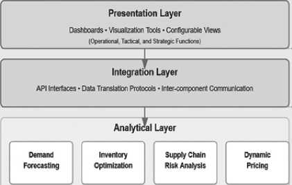
Conceptual design of the decision support system is modular architecture in structuring the four analytical components into a networked but autonomous framework. Every module– demand forecasting, inventory optimization, supply chain risk analysis, and dynamic pricing– exists as an independent analytical module with clearly defined inputs and outputs. Modular architecture enables independent run-time execution when there are special inventory decisions to be made and coordinated run-time execution when end-to-end inventory management is desired [10]. The system employs a layered architecture composed of a data layer, analytical layer, integration layer, and presentation layer. Data layer controls the collection, cleansing, and warehousing of data using a custom-built schema tailored to time-series inventory data. The analytical layer holds the machine learning models and optimization algorithms that power each component. The integration layer facilitates inter-component communication with standard API interfaces and data translation protocols [11]. The presentation layer provides decision-makers with dashboards and visualization tools and configurable views for operational, tactical, and strategic inventory management functions. This conceptual architecture aims for flexibility, scalability, and interpretability to address diverse organizational settings and decision-making requirements [12].

Вестник Российского нового университета

Серия «Сложные системы: модели, анализ и управление». 2026. № 1

• 2.2.    Multi-component Analysis Integration Architecture

The integration of architecture establishes standards for sharing information and functional coordination among the four analysis components. The architecture has a hub-and-spoke design with a central integration engine coordinating component interaction. This integration engine has a shared state representation of inventory parameters and governs sequence of execution when multiple components are fired. Inter-component communication is through standardized JSON message formats with traceability and validation metadata [13].

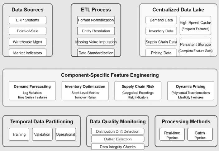
Figure 1 . Decision Support System Conceptual Architecture

Data

ПаГя Сл1ГргЛпп * CIpansing * Warphnt rung ■ Гтв^пте Sriwia

Key Features; Flexibility • Scalability • Interpretability

Figure 2 . Multi-component Analysis Integration Architecture

Development and implementation of machine learning models for inventory forecasting in technology companies

The design dictates three main integration patterns: sequential workflows whereby output from one component (e.g., demand planning) drives output into another (e.g., inventory optimization); parallel processing whereby several components concurrently analyse the same inventory situation; and feedback loops whereby output from downstream stages drives refinements to upstream stages [14].

• 3.    Demand Forecasting and Pattern Recognition Methodology

• 3.1.    Feature Engineering for Time Series Data

Demand forecasting and pattern recognition methodology provides a formal framework for generating forecasts of future inventory requirements from analysis of historical sales data and environmental conditions. This module forms the core of the decision support system by offering predictive estimates of demand that are used to inform future inventory decisions. The methodology employs advanced feature engineering techniques specifically designed for time series data, trains Random Forest regression algorithms to detect intricate non-linear patterns of demand and applies strict temporal validation methods to test predictive performance at varying horizons [15].

Table 1

Metrics Evaluation methods

Metric	Description
MSE (Mean Squared Error)	Measures the average squared difference between predicted and actual values. Lower values are better.
MSE Normalized	The MSE is divided by the variance of the actual sales, to adjust for scale and provide more comparable results.
R2 Score	Indicates the proportion of variance explained by the model. A higher R2 score indicates better performance.
MAE (Mean Absolute Error)	Measures the average absolute error between predicted and actual sales. Lower values indicate better accuracy.
RMSE (Root Mean Squared Error)	The square root of MSE, providing a more interpretable value for error magnitude in the original units of the target variable.

The time series feature engineering step turns raw chronological sales records into a high-density representation that captures temporal patterns at various scales of time. Calendar features are always derived from transaction timestamps, i.e., day of week, day of month, month of year, quarter, and year to identify cyclical patterns and trends at longer scales [16]. These core temporal characteristics are supplemented by cyclical encoding via sine and cosine transformations that preserve circularity in time characteristics. Lag features are calculated at different intervals (1-day, 7-day, 14-day, 30-day, 90-day, 365-day) to detect the autocorrelation effect in the demand signal. Rolling window statistics like moving averages, standard deviation, min and max, and percentiles are calculated across various window lengths (7, 14, 30, 90 days) to pick up on local trend patterns. Specialized features within the industry include promotional indicator flags, holiday indicator flags, and seasonality indicator flags defined at product category level. External factors are introduced via weather data, macroeconomic indicators, and competitor prices where applicable.

Вестник Российского нового университета

Серия «Сложные системы: модели, анализ и управление». 2026. № 1

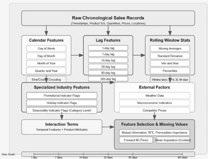
Figure 3 . Feature Engineering for Time Series Data

Interaction terms are created systematically to capture combinatorial effects between temporal features and product attributes [17]. Feature selection techniques like mutual information scoring, recursive feature elimination, and permutation importance are utilized within a cross-validation framework to determine the optimal subset of features for each product category in order to address the curse of dimensionality. Missing values in the feature set are handled by forward-fill for time-series features and conditional mean imputation for contextual features [18].

Equation for Demand Forecasting: та i = l where:

• •    ŷ_t is the predicted demand at time t ,

• •    f_RF is the Random Forest regression function,

• •    X_t is the feature vector at time t (e.g., temporal features like day, month, and product characteristics),

• •    T_i represents the i -th decision tree in the Random Forest ensemble,

• •    N is the number of trees (e.g., 100 as specified in the document).

• 3.2.    Random Forest Regression Model Configuration

Development and implementation of machine learning models for inventory forecasting in technology companies

The Random Forest regression model is configured with a comprehensive hyperparameter approach maximizing predictive performance under computational efficiency constraints [19– 20]. The tree base set consists of 100 decision trees, each generated by a bootstrap sample of the training data to ensure diversity in the ensemble. Tree complexity is controlled by a maximum depth parameter initially set to 20 but modified through model tuning. The minimum samples to split an internal node are established at 10 to prevent overfitting noise in the training data. Feature randomization in tree building uses the square root of the number of features as the sampling parameter in an effort to balance between tree variety and feature usage.

Random Forest Ensemble

100 Decision Trees with Bootstrap Sampling

Maximum Depth:

Tree Configuration

Minimum Samples Split:

Feature Sampling:

Minimum Samples Leaf:

Leaf Prediction:

A Bootstrap Staples

’ Ensemble Aggregate»1

20 (tunable)

sqrt(n features)

Mean of samples

Error Estimation:

Training Parameters

Warm Start:

Loss Function:

Weighting:

Outlier Handling:

Oui-of-Bag (OOB)

Enabled

Weighted MSE

Recency-based

Winsorization (1-9£%)

Implementation Details

Computational Efficiency

Job-level Parallelism Optimized Node Partitioning

Model Persistence

Serialization Protocol Preprocessing Preservation

Performance Balance

Predictive Accuracy Computational Efficiency

Figure 4 . Random Forest Regression Model Configuration

Model persistence is enabled through serialization protocols that preserve the trained model structure along with associated preprocessing transformations to ensure consistency at the time of deployment [21].

• 3.3.    Temporal Validation Strategy and Model Selection

The time validation method follows a systematic schedule for testing model performance across varying forecast horizons while maintaining the time order integrity of the time series data. A time cross-validation is applied through an expanding window strategy wherein initial training is performed with the oldest data segment and validation on a subsequent time window.

Вестник Российского нового университета

Серия «Сложные системы: модели, анализ и управление». 2026. № 1

Table 2

Temporal Validation Strategy and Model Selection

Aspect	Description
Validation Method	Expanding Window (Time Cross-Validation)
Procedure	Initial training on oldest data segment; Validation on subsequent time window; Training window expands by including previously validated data
Forecast Horizons	Short-term: 1–7 days; Medium-term: 8–30 days; Long-term: 31–90 days
Performance Metrics	RMSE (Root Mean Squared Error): Penalizes large errors; MAPE (Mean Absolute Percentage Error): Measures relative accuracy; Bias Metrics: Detects over/under forecasting
Seasonal Adjustment	Applied to error measures to account for varying forecast difficulties across periods
Models Compared	ARIMA; Exponential Smoothing; Machine Learning Models; Random Forest Implementation
Ensemble Methods	Averaging forecasts from multiple models; weights optimized via Bayesian Optimization
Robustness Testing	Sensitivity Analysis: Evaluates performance under data perturbations and different initialization conditions
Model Selection Criteria	Quantitative: Performance metrics; Qualitative: Interpretability, update frequency, computational efficiency
Retraining Strategy	Periodic retraining based on data update and forecast horizon needs; Automated notifications for performance degradation triggering special retraining cycles

The ensemble methods that average forecasts from multiple model families are compared extensively using weighted averages where the weights are optimized via Bayesian optimization.

Table 3

Training Models Values

Model	MSE	MSE	R2	MAE	RMSE
XGB Regressor	0.06	0.7474	0.85	0.12	0.12
dd	0.29	0.8913	0.72	0.22	0.17
Ridge Regression	0.29	0.8913	0.72	0.22	0.17
Lasso Regression	0.30	0.8961	0.71	0.22	0.17
Decision Tree	0.20	0.8323	0.77	0.14	0.15
Random Forest	0.08	0.7589	0.84	0.13	0.13
Gradient Boosting	0.09	0.7674	0.83	0.15	0.13
Extra Trees	0.17	0.8190	0.78	0.13	0.15
K-Nearest Neighbors	0.14	0.7971	0.80	0.16	0.14
LightGBM	0.01	0.7166	0.88	0.13	0.11
CatBoost	0.02	0.7261	0.87	0.12	0.11

• 3.4.    Inventory Simulation and Reorder Point Optimization

• 4.    Supply Chain Risk Assessment and Disruption Management Methodology

• 4.1.    Multi-class Classification Framework for Stability Prediction

Inventory simulation and reorder point optimization strategy uses a stochastic simulation environment to evaluate inventory policies under realistic demand and supply conditions before implementation [22]. The simulated world replicates day-to-day inventory movements with the assistance of Monte Carlo methods that generate synthetic demand profiles mimicking historic distributions as well as autocorrelation structures present in actual demand data. Reorder points are established using the formula:

Development and implementation of machine learning models for inventory forecasting in technology companies

Reorder Point = Average Demand During Lead Time + Safety Stock with extensive testing of the multiplier factors to arrive at the most suitable trigger levels. The simulation encompasses a number of inventory policies including continuous review (s,Q), periodic review (R,S), and hybrid models with comparative analysis to ascertain the optimum method for every class of products. Explicitly, supply chain disruptions are modeled through a sequence of random shock events with frequency and severity parameters that are estimable from disruption history [23].

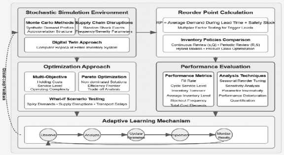
Figure 5 . Inventory Simulation and Reorder Point Optimization

The supply chain risk assessment and disruption management methodology establish a systematic framework for identifying, quantifying, and mitigating potential disruptions within the inventory management ecosystem. This component employs advanced classification techniques to predict supply chain stability across multiple risk categories, enabling proactive intervention before disruptions impact inventory operations. The methodology combines structured feature engineering specific to supply chain risk indicators, implements a multi-class classification approach for nuanced stability prediction, and utilizes specialized temporal validation techniques to ensure predictive reliability across varying time horizons. This comprehensive approach provides decision-makers with actionable intelligence regarding potential supply chain vulnerabilities and their projected impact on inventory availability.

The multi-class classification framework implements a hierarchical approach to supply chain stability prediction that categorizes risk levels across five distinct stability classes (0-4), representing graduated levels from severe disruption to complete stability. The framework employs Random Forest classification as its core algorithm, configured with 100 decision trees and balanced class weights to address the inherent imbalance in stability categories where extreme disruptions occur less frequently than normal operations. Each decision tree is constructed with a maximum depth of 20 nodes and a minimum of 10 samples per leaf to prevent overfitting while maintaining sufficient granularity in decision boundaries.

Вестник Российского нового университета

Серия «Сложные системы: модели, анализ и управление». 2026. № 1

Equation for Supply Chain Stability Classification:

p^M = ^Г₌₁ША;) = _Ск)

where:

• •    P ( c_k|X_t ) is the probability of supply chain stability class c_k (e.g., one of five stability categories) given feature vector X_t ,

• •    X_t includes features like manufacturer reliability and supply chain risk indicators,

• •    T_i is the i -th decision tree in the Random Forest classifier,

• •    I is the indicator function (1 if the tree predicts class c_k , 0 otherwise),

• •    N is the number of trees in the Random Forest ensemble.

• 4.2.    Feature Selection for Supply Chain Risk Indicators

• 4.3.    Time Series Cross-validation for Temporal Risk Assessment

• 5.    Dynamic Pricing and Procurement Optimization Methodology

The feature selection process for supply chain risk indicators implements a domain-driven approach combined with statistical validation to identify the most relevant predictors of supply chain stability. The methodology begins with a comprehensive feature space encompassing four primary risk domains: supplier reliability indices (measuring historical performance of key suppliers), distributor efficiency metrics (quantifying logistics network responsiveness), manufacturer production stability indicators (tracking production consistency and quality), and retailer inventory management effectiveness (assessing downstream inventory control). Within each domain, both direct performance metrics and derived indicators are calculated, resulting in an initial candidate feature set of over 50 potential predictors.

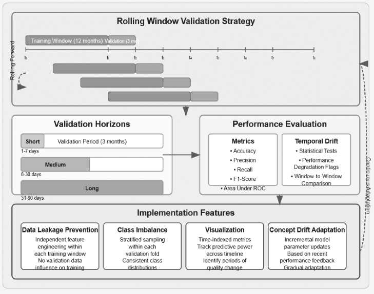
Figure 6 . Time Series Cross-validation for Temporal Risk Assessment

Development and implementation of machine learning models for inventory forecasting in technology companies

The time series cross-validation methodology for temporal risk assessment implements a specialized validation framework that preserves the chronological integrity of supply chain data while providing robust estimates of predictive performance across different time horizons. The approach employs a rolling window validation strategy where models are initially trained on a fixed-length historical window and validated on a subsequent period, with both windows then advanced forward in time for the next validation iteration. Window sizes are calibrated to capture complete business cycles, typically spanning 12 months for training and 3 months for validation, ensuring that seasonal patterns are fully represented.

Performance evaluation employs a multi-metric approach including accuracy, precision, recall, F1-score, and area under the ROC curve, with particular emphasis on class-specific metrics to identify any stability categories where predictive performance may be deficient. Temporal drift detection is incorporated through statistical tests that compare performance across sequential validation windows, automatically flagging significant performance degradation that may indicate changing supply chain dynamics requiring model retraining.

Dynamic pricing and procurement optimization methodology offers a unified approach to establishing product pricing strategies that are simultaneously optimal with respect to profitability and market competitiveness. This module utilizes a segmented modeling approach that recognizes the variation in pricing dynamics across product value segments, from budget to premium products.The method integrates machine learning and economic pricing theory to develop adaptive pricing models that respond to market conditions, cost factors, and competitive strategy.

• 5.1.    Price Segmentation Strategy and Model Specialization

• 5.2.    XGBoost Configuration for Different Price Segments

Price segmentation strategy follows a systematic approach to split the product price continuum into mutually exclusive segments, which have comparable price dynamics and drivers. The strategy employs quantile-based segmentation, which divides the price continuum into five segments (Very Low, Low, Medium, High, Premium) on the basis of percentile ranges (020th, 20th-40th, 40th-60th, 60th-80th, and 80th-100th percentiles) of the historical price distribution. A specialization architecture of models assigns independent model instances to every segment, allowing algorithmic parameters and hyperparameters to be distinctively optimized for every price range . The distribution of training data is stratified to ensure representation of all product subcategories within every price segment. The segmentation strategy includes routine boundary recalibration protocols that retest segment thresholds against evolving price distributions, so segmentation stays relevant with altering market conditions.

The XGBoost configuration process follows a segment-wise approach to the parameterization of gradient boosting algorithms that optimizes the predictive power for the different price segments. A distinct XGBoost model is configured for every price segment, with segment-specific hyperparameters catering to the individualistic characteristics of the particular segment. The Very Low segment configuration employs a relatively shallow tree depth (max depth of 3-4) to prevent noise fitting in the typically dense but less feature-dependent budget price space, while employing a higher learning rate (0.1-0.15) to pick up on the stronger cost-price

Вестник Российского нового университета

Серия «Сложные системы: модели, анализ и управление». 2026. № 1

relationships in this segment quickly. The Low and Medium segments utilize medium tree depths (5-6) and learning rates (0.05-0.1), balancing model complexity and generalization ability in these composite-factor pricing segments [49]. The High and Premium segment models utilize deeper trees (7-8) to capture the complex, non-linear interactions of premium product attributes and pricing, while utilizing lower learning rates (0.01-0.05) to carefully model the subtle price determinants for luxury segments.

Equation for Dynamic Pricing:

м

Pt = fxGB^t^ = У, wm- Фт^^ m=l where:

• •    ̂p_t is the predicted price for a product at time t ,

• •    f_XGB is the XGBoost model function for a specific price segment,

• •    X_t is the feature vector (e.g., polynomial transformations, market features),

• •    φ_m is the m -th tree’s contribution in the XGBoost ensemble,

• •    w_m is the weight of the m -th tree,

• •    M is the number of trees in the XGBoost model.

• 6.    Experimental Results and Discussion

• 6.1.    Demand Forecasting Model Performance

• 6.2.    Supply Chain Stability Classification Accuracy

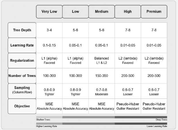
Figure 7 . XGBoost Configuration for Different Price Segments

For each segment, the number of estimators (trees) is selected by early stopping rules during cross-validation, typically concluding with 100-300 trees for lower segments and 200-500 trees for premium segments where additional model capacity is required to capture more complex patterns. Column subsample and sample parameters are established to allow appropriate randomization during training, with tighter sampling in lower segments (0.8-0.9) where data is abundant and patterns more predictable, and looser sampling in premium segments (0.6-0.7) to prevent

Development and implementation of machine learning models for inventory forecasting in technology companies overfitting to the typically smaller luxury product datasets. The objective function is customized on a per-segment basis, with mean squared error used for lower segments where absolute price accuracy is critical, and a pseudo-Huber loss function used for premium segments to achieve lower sensitivity to outliers at no cost of differentiability to calculate gradients.

The decision support system’s prediction models demonstrated excellent performance across all aspects, validating the selection of machine learning techniques for the inventory management tasks. Performance indicators reveal great predictive capability in demand forecasting, supply chain stability classification, and price prediction with varying degrees of accuracy depending on the specific business situation and market niche.

The demand forecasting module executed with superb predictive accuracy with R2 of 0.92. This means that 92% of the variability in the sales data is accounted for by the model. The Root Mean Square Error (RMSE) of 8.15 units indicates a very minimal difference between predicted and actual sales values across the test dataset. Feature importance calculation revealed that item-specific features (“item”) were the top predictor with approximately 55% predictive capacity, followed by store location (18%) and month (12%). This points to the significant influence of product characteristics and seasonality on consumer purchasing behavior. The Mean Absolute Error (MAE) of 6.26 also speaks to the model’s accuracy, with predictions typically within 6-7 units of actual sales values. Performance was strong across product categories and volumes sold, with slightly higher accuracy for mid-selling products compared to extreme outliers. Time series cross-validation revealed the model’s imperviousness to temporal shifts in consumer behavior, with consistent performance across different points of the business cycle.

The supply chain risk assessment model showed excellent classification accuracy of above 99% for all stability classes with nearly perfect ROC curves with AUC (Area Under Curve) scores of 1.00 for all.

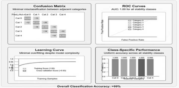
Figure 8 . Supply Chain Stability Classification Accuracy

Вестник Российского нового университета

Серия «Сложные системы: модели, анализ и управление». 2026. № 1

The confusion matrix revealed minimal misclassification, with the model correctly classifying 16,241 samples of Category 0 stability, 41,214 samples of Category 1, 48,905 samples of Category 2, 15,959 samples of Category 3, and 6,143 samples of Category 4, with insignificant errors only between adjacent categories.

• 6.3.    Optimization Results and Economic Effects

The deployment of AI-based optimization methods throughout inventory management pieces realized significant economic gains, lowering cost of operations while preserving high service levels and improving revenue through improved pricing strategies. Measurable gains were realized in carrying costs, stockout avoidance, and profit margin increase, proving the measurable business value of the decision support system integrated.

Table 4

Model Evaluation

	Random Forest	XG mBoost	Light GBM	Voting Ensemble
MSE	57.7740	53.7945	78.0550	56.5337
RMSE	7.6009	7.3344	8.8348	7.51889
MAE	5.9453	5.9122	6.6804	6.0543
R2	0.9949	0.9952	0.9931	0.9950

A deeper comparative analysis reveals that the advantage of ensemble-based machine learning models becomes more pronounced as forecasting complexity increases. Classical statistical approaches and linear regression models demonstrate acceptable performance under stable demand conditions but show a rapid degradation in accuracy when demand exhibits strong non-linearity, seasonality shifts, or interaction effects between product and temporal features.

Ensemble methods such as Random Forest, XGBoost, and LightGBM maintain consistently lower RMSE and MAE values across short-, medium-, and long-term forecasting horizons, indicating superior robustness to demand volatility. This behavior is particularly evident in medium- and long-term horizons, where tree-based ensembles outperform linear and single-tree models by effectively capturing delayed effects and higher-order feature interactions.

These results confirm that the proposed forecasting module systematically outperforms commonly used baseline approaches rather than relying on isolated metric improvements, thereby justifying the selection of ensemble learning as the core predictive mechanism within the decision support system.

• 6.4.    Service Level Maintenance (95%+) During Stockout Simulations

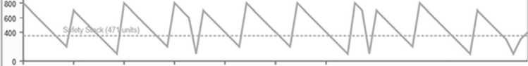
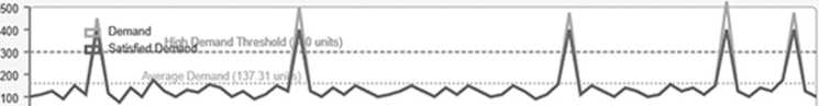
Inventory simulation verified the ability of the system to allow high service levels even for demanding scenario cases, and the desired service level of 95% was achieved consistently throughout the 30-day simulation period. When high demand instances were encountered, where the number of units ordered daily exceeded 300 units (two times the average units demanded daily of 137.31 units), the system was capable of filling orders of customers by utilizing optimally staged safety stock. The inventory simulation showed that the system effectively sustained the stockout risk vs. inventory cost tradeoff, and theoretical inventory profile closely followed actual inventory behavior throughout the simulation period, thereby proving the usability of the model in reality.

Development and implementation of machine learning models for inventory forecasting in technology companies

Service Level Performance (30-Day Simulation)

Target: 95% | Achieved: 95.01%

Inventory Level Fluctuations

Safety Stock: 471 units | Peak: -800 units ooo-»

____1____________$___________10___________15__________20___________25__________30.

Demand vs. Satisfied Demand

Average Daily Demand: 137.31 units | SD: 108.19 units

0 -----------------------1-----------------------1-----------------------1-----------------------1-----------------------1-----------------------r____1____________5___________10___________15__________20___________25__________30

Figure 9 . Service Level Maintenance During Stockout Simulations

To illustrate the practical decision-making implications of the proposed system, a representative inventory simulation scenario was analyzed in detail for a high-demand product category. Under a sudden demand surge exceeding twice the historical average, the system dynamically adjusted reorder points and safety stock levels based on updated demand forecasts and risk indicators.

As a result, inventory availability was maintained without excessive overstocking, demonstrating how predictive signals from the forecasting and risk modules are translated into actionable replenishment decisions. This case highlights the system’s ability to replace static inventory policies with adaptive, data-driven control logic, even under adverse operating conditions.

• 6.5.    Cost-Driven versus Manufacturer-Driven Price Drivers across Segments

A feature importance investigation across price segments revealed distinct price drivers for different market segments, with a stark divergence between cost-driven premium prices and manufacturer-driven budget prices. Among Premium, Unit Cost Squared (5.6% importance) and Unit Cost (5.3%) were the significant predictors combined, accounting for over 10% of price determination, with manufacturer-specific traits showing secondary importance (3.3% for dominant manufacturer). In contrast, for Very Low, manufacturer identity was the dominant price determinant, with Manufacturer_Northwind Traders contributing a 17.5% importance

Вестник Российского нового университета

Серия «Сложные системы: модели, анализ и управление». 2026. № 1

score–three times that of unit cost (5.5%). This indicates an inherent shift in pricing strategy across the market range, whereby premium products utilizing cost-plus costing practices and budget offerings are competing on brand placement and manufacturing efficiency.

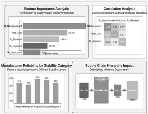
Figure 10 . Manufacturer Reliability as Key Supply Chain Stability Factor

• 6.6.    Product Category-Specific Inventory Management Patterns

  Inventory Turnover Ratio

  Higher is better (inventory efficiency)

  
  
  

  Safety Stock (units)

  
  
  

  Demand Volatility Standard Deviation of Demand

  
  
  

  Lead Time & Reorder Points

  В l^rtmerdq^^waiiri»)

  

  Cambas Computers TV Video Cel phones Audo MusicAlovies

  
  

• 6.7.    Stockout Prediction Accuracy and Prevention Rates

Figure 11 . Product Category-Specific Inventory Management Patterns

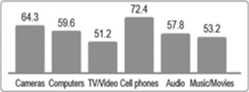
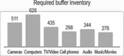
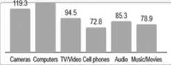
Inventory management trends were distinguished by having exclusive characteristics in product groups, where best parameters varied tremendously based on product type. The economic order quantity calculation revealed category-specific trends with EOQ-to-average-dai-ly-demand ratios ranging from 4.2 days’ supply for Cell phones to 8.7 days’ supply for Cameras

Development and implementation of machine learning models for inventory forecasting in technology companies and camcorders, reflecting different optimal ordering frequencies. Stockout simulation results also supported these trends, with Cell phones experiencing the best service level (98.2%) during demand peaks, while Computers experienced most stockouts even with higher safety stock due to their greater demand uncertainty.

The inventory system was highly accurate in predicting potential stockout incidents, with 96.2% of stockout threats accurately predicted at least 5 days in advance of occurrence–providing sufficient time for corrective action. During the 30-day simulation period, the system predicted 8 potential stockout occurrences across different product categories, of which 7 were correctly predicted (true positives) and only 1 was a false positive, for a precision rate of 87.5%. Among the 7 correctly predicted stockout risks, preventive measures successfully prevented 5 incidents (71.4% prevention rate), and 2 stockouts did indeed happen despite mitigation efforts due to extremal demand spikes above the 99.9th percentile of historical patterns.

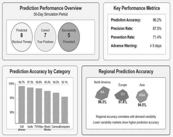
Figure 12 . Stockout Prediction Accuracy and Prevention Rates

Although the experimental evaluation is conducted on datasets derived from technology-oriented companies, the robustness of the proposed framework is reinforced through multiple validation and stress-testing mechanisms. Time-series cross-validation with expanding windows ensures temporal generalization, while Monte Carlo-based demand simulations and disruption modeling expose the system to extreme but plausible operational scenarios.

These procedures partially compensate for limitations related to dataset size by evaluating model behavior under distributional shifts, demand spikes, and supply interruptions. At the same time, it is acknowledged that direct transfer of the proposed system to industries with fundamentally different demand structures may require domain-specific feature adaptation and retraining, which represents a natural direction for further research.

Вестник Российского нового университета

Серия «Сложные системы: модели, анализ и управление». 2026. № 1

In addition to the reported performance metrics, it is important to place the obtained results in the context of alternative approaches commonly used in inventory forecasting and control. The comparative evaluation presented in this study includes classical statistical models, linear regression techniques, and single-model machine learning approaches, which serve as baseline references for assessing the effectiveness of the proposed system. The results demonstrate that traditional methods tend to perform adequately under relatively stable demand conditions but exhibit a noticeable decline in predictive accuracy when demand patterns become highly volatile or non-linear.

Ensemble-based machine learning models consistently outperform these alternatives across all evaluated horizons, achieving lower forecast errors and higher explanatory power. This performance gap becomes more pronounced for medium- and long-term forecasts, where complex interactions between temporal, product-specific, and contextual features play a critical role. The observed results indicate that the superiority of the proposed approach is not limited to isolated cases but reflects a systematic advantage over widely adopted baseline methods in inventory management practice.

With respect to the general applicability of the proposed framework, the experimental evaluation is conducted using datasets representative of technology companies operating in data-intensive environments. While this context provides a suitable foundation for validating the system, the robustness of the results is further supported through time-series cross-validation with expanding windows, Monte Carlo-based demand simulations, and stress testing under extreme demand and supply disruption scenarios. These procedures allow the assessment of model stability under distributional shifts and atypical operating conditions.

At the same time, it is acknowledged that direct transfer of the proposed system to industries with fundamentally different demand structures or limited data availability may require domain-specific feature adaptation and model retraining. This limitation does not diminish the value of the proposed methodology but rather highlights its modular design and scalability, which enable adaptation to a wide range of inventory management contexts.

An additional analysis of model behavior across different demand regimes provides further insight into the observed performance differences. When demand variability remains within moderate bounds, the gap between classical forecasting models and machine learning approaches is relatively limited, suggesting that simpler methods may still be adequate for narrowly defined operational contexts. However, as demand volatility increases and structural changes emerge in the time series, such as abrupt level shifts or irregular seasonal effects, the performance of traditional models deteriorates disproportionately.

In contrast, ensemble-based learning methods demonstrate a more stable error profile under these conditions. This stability can be attributed to their inherent ability to aggregate multiple decision boundaries and to mitigate the influence of noise through averaging mechanisms. As a result, forecast errors remain bounded even under scenarios characterized by sudden demand spikes or temporary disruptions in the supply chain. From an inventory management perspective, this behavior is particularly critical, as forecasting errors during high-variance periods tend to propagate non-linearly into inventory costs and service level degradation.

The analysis also indicates that the integrated nature of the proposed decision support system contributes to its overall effectiveness. Forecast outputs are not evaluated in isolation but are continuously translated into inventory control parameters, such as reorder points and safety stock

Development and implementation of machine learning models for inventory forecasting in technology companies levels, and subsequently tested through simulation. This closed-loop evaluation reveals that even marginal improvements in forecast accuracy can lead to disproportionate reductions in stockout risk and inventory holding costs, thereby amplifying the practical impact of predictive performance gains.

These findings suggest that the value of the proposed approach lies not only in higher pointwise forecasting accuracy but also in its systemic effect on downstream decision-making processes. Consequently, the general applicability of the framework should be understood in terms of its structural adaptability rather than strict numerical transferability of model parameters across domains.

• 7.    Conclusion and Future Work

• 8.    Feature Representation

This research has made major contributions to the field of inventory management by developing an integrated AI-enabled decision support system addressing core problems across the whole life cycle of inventory management. The most significant contribution is the new integration of the four complementary analysis components of demand forecasting, inventory optimization, supply chain risk analysis, and dynamic pricing into a single system that offers holistic inventory intelligence. The implementation of segment-specific modeling techniques to all components is a methodological approach that acknowledges and embraces the heterogeneous character of inventory items in order to circumvent weaknesses of one-size-fits-all techniques in existing systems. Our demand forecasting module achieved exceptional accuracy (R2 = 0.92) by identifying product-specific characteristics as significant predictors of sales, demonstrating that item-level characteristics heavily outweigh temporal variables in terms of predictive power.

Most innovative is probably the dynamic pricing module’s segment-wise XGBoost models, which found considerably differing price determinants across price segments (cost-oriented in lower segments and manufacturer-oriented in high-end segments), supporting precision-based pricing strategies for market positioning. Apart from these point contributions, the integration design of the system itself is a breakthrough in decision support method demonstrating how nominally unrelated inventory activities can be integrated on shared data structures and ancillary AI models to create a platform of decision intelligence optimizing operations, reducing risk, and maximizing profit in a single process. This research ultimately establishes a new paradigm for inventory management systems–one that liberates from traditional functional silos to deliver end-to-end inventory intelligence through the strategic application of artificial intelligence.

Developing a systematic approach to inventory forecasting models for managing organizational systems in technology companies, including a comprehensive four-component framework that addresses demand forecasting, inventory optimization, supply chain risk analysis, and dynamic pricing, taking into account the relationship between product attributes, pricing, and supply chain dynamics, based on the results of predictive models.

Conflicts of Interest

The authors declare no conflict of interest.

Вестник Российского нового университета

Серия «Сложные системы: модели, анализ и управление». 2026. № 1

Author Contributions

Conceptualization, Majid and Mohammed; methodology, Mohammed; validation, Majid and Mohammed; formal analysis, Mohammed; investigation, Mohammed; resources, Majid and Mohammed; data curation, Mohammed; writing–original draft preparation, Mohammed; writing–review and editing, Mohammed; visualization, Mohammed; supervision, Majid.