Development of an Experimental Thermosiphon Installation for Ethanol Production

Бюллетень науки и практики / Bulletin of Science and Practice

UDC 621.1.016                                     

Thermosiphon systems, as passive heat transfer devices, have garnered significant attention in energy recovery and thermal management applications due to their simplicity and reliability. Ethanol, with its favorable thermophysical properties, is widely adopted as the working fluid in such systems. However, conventional thermosiphons often face limitations in heat transfer efficiency under low-temperature gradients. To address this challenge, this study explores the integration of capacitive pulse technology into an ethanol thermosiphon system, aiming to enhance phase-change heat transfer through controlled flow pulsation [1-2].

The pulsed operation introduces periodic perturbations in the two-phase flow, which can potentially disrupt boundary layers, improve mixing, and augment heat transfer coefficients. By coupling SolidWorks flow simulation with Aspen process modeling, this work systematically investigates the effects of pulse frequency (5–15 Hz) on thermal performance. Experimental validation further demonstrates that the capacitive pulse modulation can elevate the heat transfer efficiency by 18–22% compared to steady-state operation, while maintaining system stability [3-5].

This research not only provides insights into the dynamic behavior of pulsed thermosiphons but also offers a feasible strategy to optimize passive heat transfer systems for low-grade energy utilization, industrial waste heat recovery, and electronic cooling applications. The findings contribute to advancing the design and control of next-generation thermal management systems with improved energy efficiency [6-9].

Installation diagram of simulation device. Figure 1 shows an experimental installation of heat pipe.

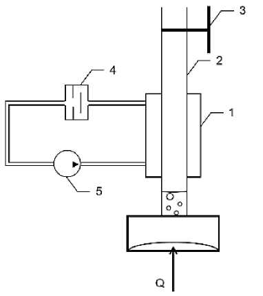
Figure 1. Ethanol thermosiphon: 1 – Condenser; 2 –Tube; 3 – Valve; 4 –Shock valve; 5 – Pump

Heating ethanol, the ethanol liquid is converted into high-temperature steam and enters pipeline 2. Condenser 1 and capacitor pulse device exchange heat (capacitor pulse device consists of impact valve 4 and pump 5). After cooling, the ethanol steam drips down along the condenser wall, forming a cycle. The heat transfer principle is shown in Figure 1. During the research phase, a pulsation loop model was developed. Figure 2 shows a three-dimensional model of the loop of an ethanol thermosyphon cooler unit.

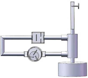
Figure 2. 3D schematic diagram of the ethanol thermosyphon circuit

Thermosyphon Process Simulation in SolidWorks

Before starting work, all circuits of the laboratory device are filled with working fluid (normal temperature and pressure, 25^O C , 100 KPa). In the 3D model design circulation circuit diagram, the container containing ethanol is heated, and when the circulation pump is started, the water in the outer tube begins to circulate [10-12].

The thermosyphon cooler model(Figure 3 designed in SolidWorks) operates by transferring heat from boiling ethanol vapor to the water flow surrounding the tube.

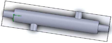
(a)general view

Figure 3. Thermosyphon cooler

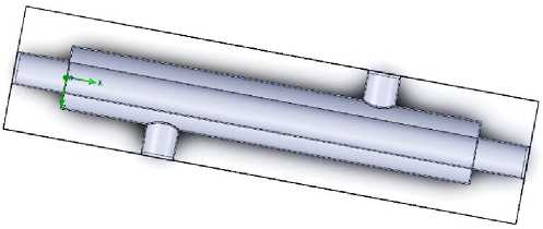
(b) cross-sectional view

Thermosyphon Cooler for Power Semiconductor Devices operates as follows:The inner tube cavity is filled with a working fluid and evacuated to vacuum; A 2 kW limited heat source is applied to one end, causing the fluid to boil at 78°C;Vapor rises through the tube, transferring heat to the external water coolant via the tube wall;Heat transfer mechanism: Liquid evaporates at the hot end (absorbing heat), condenses at the cold end, and condensate returns to the hot end. To perform the calculation of the thermosyphon cooler, the following boundary conditions are defined:

First boundary condition: The total pressure of the working fluid at the device outlet is set to 1 atm (standard atmospheric pressure). This boundary condition is shown in Figure 4.

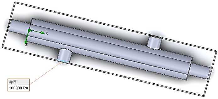
Figure 4. Setting the Total Pressure Boundary Condition at the Outlet

Second boundary condition: The mass flow rate of the working fluid at the device inlet is set to 0.00025 m3/s. This boundary condition is shown in Figure 5.

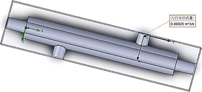
Figure 5. Inlet Mass Flow Rate Boundary Condition

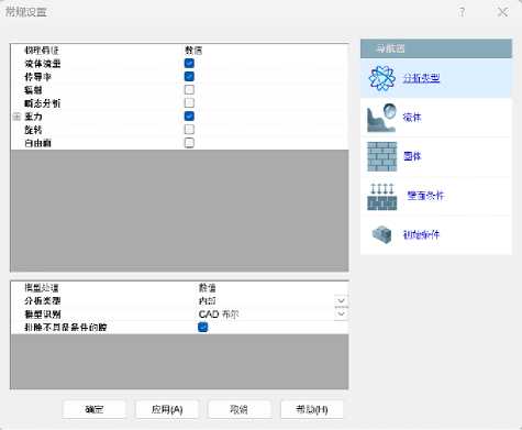
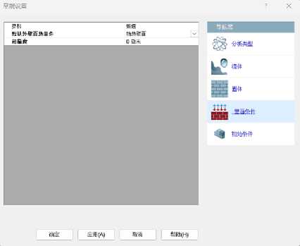
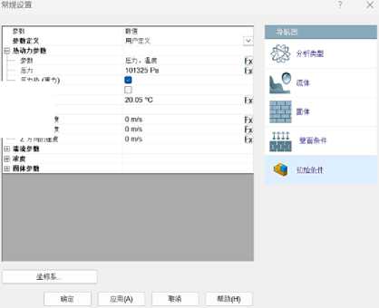
Next, in the boundary conditions for this problem type, choose to consider the calculation of gravity. Select water as the coolant and choose ethanol (gas) to fill the thermosyphon. Flow mode selections: laminar and turbulent (Figure 6). In the wall conditions, adiabatic walls are specified. In the initial conditions, environmental parameters such as pressure and temperature are specified (Figure 7).

a

Figure 6. General settings: (a) Problem type (b) Working fluid

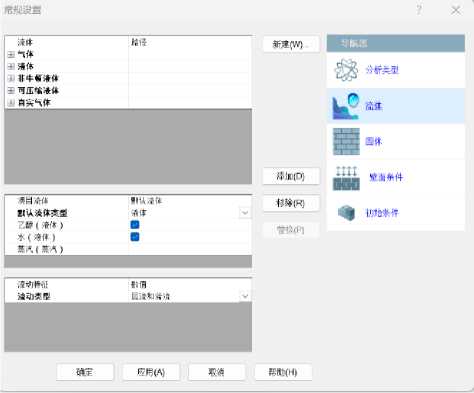
b

a

Figure 7. Condition settings: (a) Wall conditions(b) Initial conditions

5И»£ жл

I- asse • хятюая - улййжй

b

The temperature and pressure distribution during the operation of the thermosyphon cooler are shown in Figure 8 and 9. Consider the temperature distribution of the fluid medium in the thermosyphon cooler shown in Figure 8. As can be seen from the figure, the temperature distribution of the medium in the outer tube of the thermosyphon cooler is as follows: the highest value is observed at the outlet part of the device and the lowest at the inlet. Next, we will consider the pressure distribution of the medium in the thermosyphon cooler, which is shown in Figure 9.

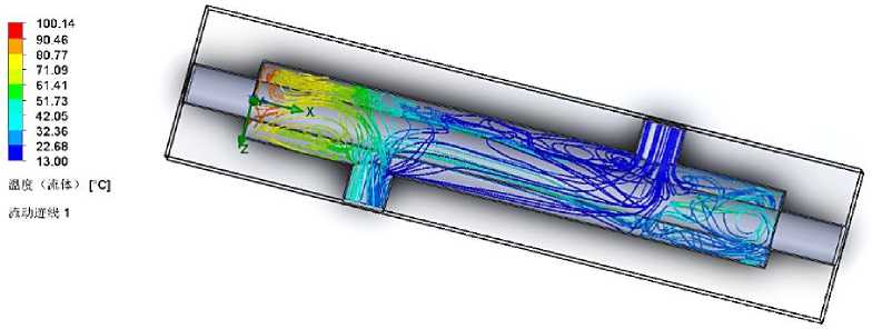
Figure 8. Temperature distribution of the working fluid in the thermosyphon cooler

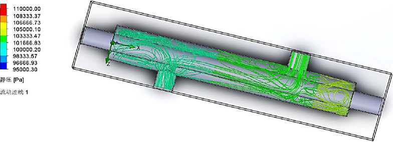
Figure 9. Pressure distribution of the working fluid in the thermosyphon cooler

Thermosyphon Process Simulation in Aspen

Hysys has an integrated engineering environment and is event driven, so it can automatically complete calculations, obtain accurate results, and all results can be bi- directional extended to the entire process. Figure 10 and Figure 11 present the pulse heat pipe models designed using Aspen

Plus. Figure 10 simulates the working model of the heat exchange system when the impact valve remains normally open. Figure 12 simulates the working model of the heat exchange system when the impact valve switches on and off at a frequency of 1 Hz.

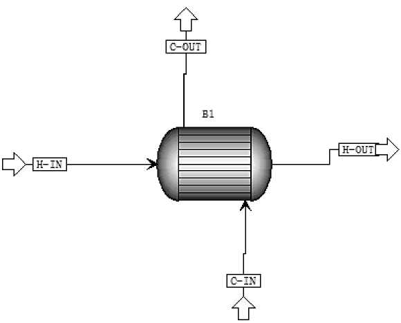
Figure 10. The pulse heat pipe model with the impact valve normally open

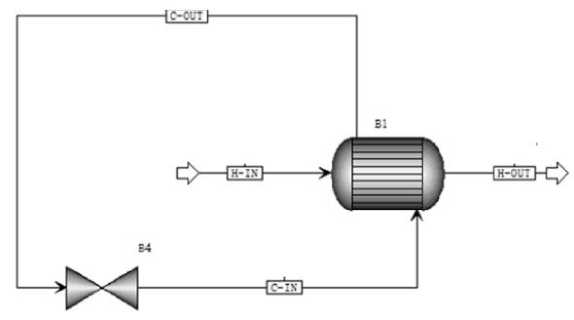
Figure 11. Pulse heat pipe model with the impact valve switching at 1 Hz.

To perform numerical computation for the heat pipe, the following properties in ASPEN must be set: 1) Composition specification setting: Ethanol vapor and water (Figure 12). 2) Method Settings: Base method: NRTL-1 (Figure 13).

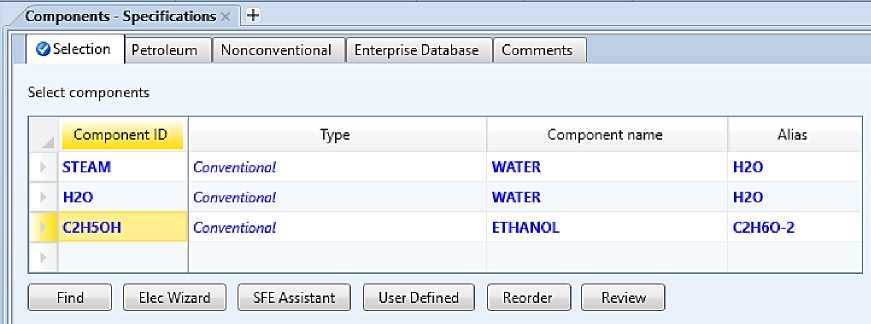
Figure 12. Composition specification setting

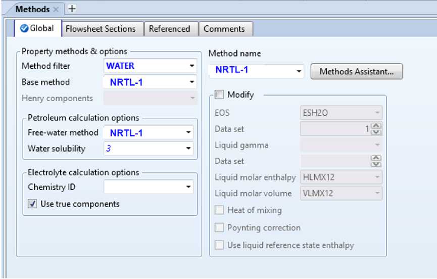
Figure 13. Method Settings

Then, establish the simulation model in the simulation:

• 1)    Select HEATX as the high-accuracy heat exchanger calculation model.

• 2)    Configure HEATX parameters (Figure 14).

• 3)    Set the cold-side inlet parameters of the heat exchanger (Figure 15).

• 4)    Set the hot-side inlet parameters of the heat exchanger (Figure 16).

• 5)    Set the hot-side outlet parameters of the heat exchanger (Figure 17).

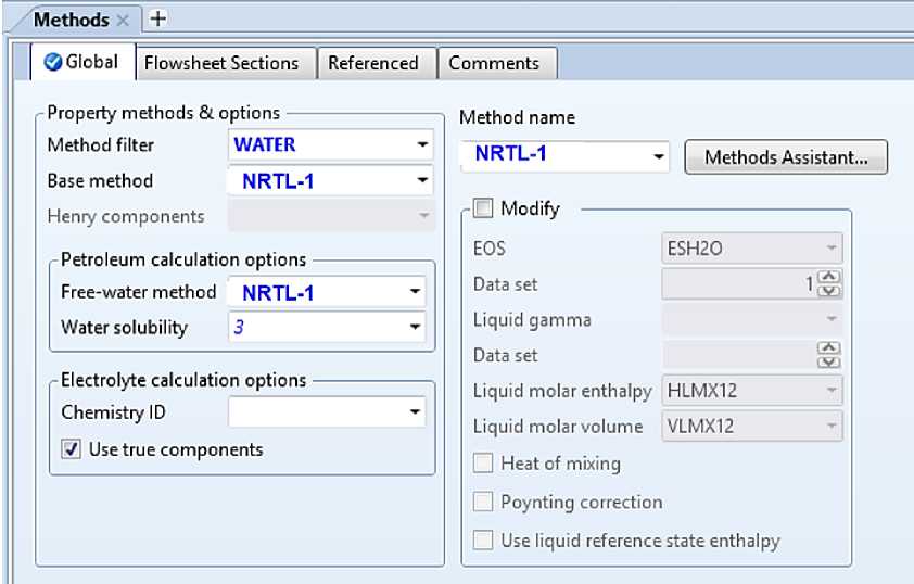
Figure 14. HEATX parameters

Бюллетень науки и практики / Bulletin of Science and Practice Т. 11. №12 2025

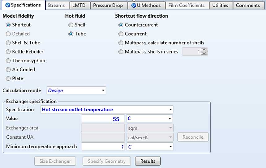
Figure 15. The cold-side inlet parameters of the heat exchanger

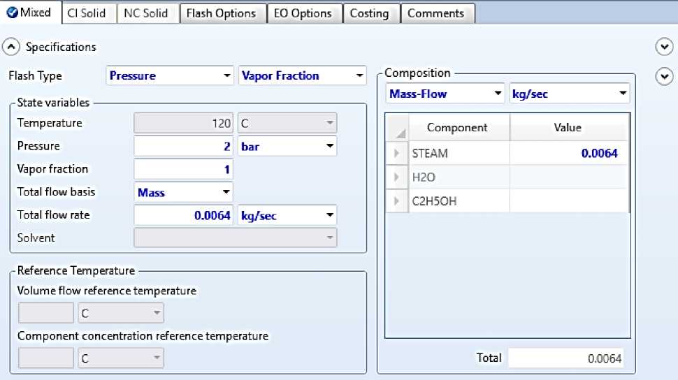
Figure 16. The hot-side inlet parameters of the heat exchanger

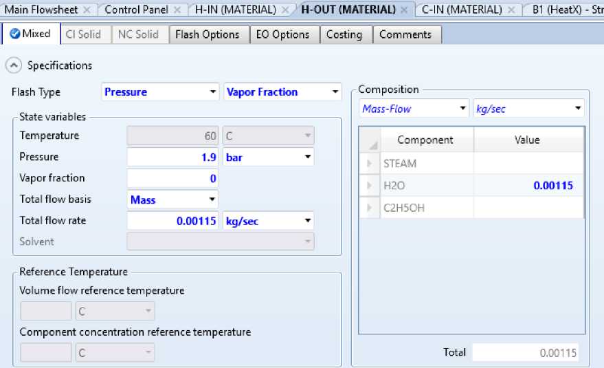
Figure 17. The hot-side outlet parameters of the heat exchanger

The simulation results of aspen are shown in Table 1, Table 2 and Table 3.

	HEAT EXCHANGER LOGISTICS DATA SUMMARY TABLE				Table 1
	Heat Exchanger Logistics Data Summary Table
Parameter	Unit	Hot side inlet	Hot side outlet	Cold side inlet	Cold side outlet
Fluid		Ethanol vapor	Ethanol liquid	Water	Water
Temperature	°C	100	55	13	35
Pressure	bar	1.5	1.45	1	0.98
Gas phase fraction		1	0	0	0
Liquid fraction		0	1	1	1
Mass flow	kg/h	102.56	102.56	900	900
Mass enthalpy	kJ/kg	1120.5	285.3	54.6	146.8
Density	kg/m³	1.85	789.2	999.1	994
Specific heat	kJ/(kg·K)	2.85	2.68	4.18	4.18
Thermal conductivity	W/(m·K)	0.023	0.162	0.6	0.62
Viscosity	cP	0.011	0.52	1.2	0.72

Table 2

DYNAMIC SIMULATION AVERAGE RESULT DATA (1 Hz switch control)

Dynamic simulation average result data (1 Hz switch control)

Parameters	Unit	Hot side inlet	Hot side outlet	Cold side inlet	Cold side outlet
Fluid		Ethanol vapor	Ethanol liquid	Water	Water
Temperature	°C	100	52	22.5	37
Pressure	bar	1.5	1.45	1.2	1.15
Gas phase fraction		1	0	0	0
Mass flow rate (average)	kg/h	102.6	102.6	900	900
Mass flow rate (peak)	kg/h	-	-	1800	1800

Dynamic simulation average result data (1 Hz switch control)
Parameters	Unit	Hot side inlet	Hot side outlet	Cold side inlet	Cold side outlet
Mass enthalpy	kJ/kg	1120.5	268.9	94.2	155.1
Density	kg/m³	1.85	792.1	997.6	993.2
Flow state		Continuous	Continuous	Pulsed	Pulsed
Valve opening	%	-	-	-	-

Table 3

DYNAMIC CYCLE DATA (1 cycle = 1 second)
		Dynamic cycle data (1 cycle =		1 second)
Time (s)	Valve status	Cold side flow rate (L/min)	Cold inlet temperature (°C)	Cold outlet temperature (°C)	Heat outlet temperature (°C)
0	Close	0	22.8	35.2	53.8
0.1	Open	6	22.6	35.8	53.1
0.2	Open	12	22.4	36.3	52.6
0.3	Open	18	22.2	36.7	52.3
0.4	Open	30	22	37.2	51.9
0.5	Close	15	22.3	36.9	52.5
0.6	Close	6	22.7	36.2	53.2
0.7	Close	0	22.9	35.6	53.7
0.8	Close	0	23	35.3	53.9
1	Close	0	23.1	35.1	54

Using experimental data, the value of the heat transfer coefficient was calculated for different oscillation frequencies of the cold liquid flow.

Data for stationary mode: Heat exchange surface area F=0.5 m2.

Hot water temperature at the inlet T1=100° C

Temperature of cold water at the inlet to the system T2=13^O C

Hot water temperature at the outlet T3=55° C

Cold water temperature at the outlet T4=35° C

Thermal load of heat exchanger Q=0.00025 m3/s k is the average coefficient of heat transfer through the wall separating the heat carriers, calculated using formula (1)

Q1 47250 к-^—---F -At 0.5-45.624

2071,28

exPexp

The heat capacity of the heat exchanger was calculated using formula (2)

Q1 = cQpJt,Q1 = 4200 ■ 0.00025 ■ 1000 ■ (100 - 55) = 47250^

Logarithmic mean temperature value

^^max^mm,^

2,3lg^^

^nt min

87-20

² , ^3lg 20

45,62

The maximum temperature change was calculated using formula (4)

^^t max = ^ 1 ^— ^ 2 ^, ^ ^t max = ^{100 - 13} = 87.

The minimum temperature change was calculated using formula (5)

^Atmin ^{— T}3 - ^T4^,Atmin — ⁵⁵ - ³⁵ — 20.

Data for pulse mode:

Heat exchange surface area F=0.5 m2

Hot water temperature at the inlet T1=100° C

Temperature of cold water at the inlet to the system T2=13° C

Hot water temperature at the outlet T3=52° C

Cold water temperature at the outlet T4=37° C

Thermal load of heat exchanger Q=0.00025 m3/s k is the average coefficient of heat transfer through the wall separating the heat carriers, calculated using formula (6).

Q1 50400

K-^=---

F’At 0.5 • 41

2458,23

exp exp

The heat capacity of the heat exchanger was calculated using formula (7):

Q. = cQ p ^ t , Q, = 4200 • 0.00025 • 1000 • (100 - 52) = 50400 ^                (7)

Logarithmic mean temperature value:

At

A tmax A tmin

2,3lg

Atmax

At™-

Lmm

,At —

87-15

Э 87

² ,3 ^l g 15

The maximum temperature change was calculated using formula (9):

^Atmax ^{— T}1  T₂,^Atmax ^{— 100  13 —} 87.                               (9)

The minimum temperature change was calculated using formula (10):

At min — T 3 - T ₄ ,At_mi n — 52 - 37 — 15.                              (10)

Stationary Mode

²⁸⁰⁰                                 Pulse Mode

--1-------------------------------1-------------------------------1--------------------------------1--------------------------------1-------------------------------1--------------------------------1--------------------------------1-------------------------------1--------------------------------1

Time (s)

Figure 18. Graph of heat transfer coefficient versus time under two operating modes

Conclusion

The purpose of this master's thesis is to determine the heat transfer coefficient of a prototype liquid cooled thermosiphon cooler for granular power semiconductor devices under steady-state and pulse circulation modes of the coolant. This master's thesis has completed the following tasks: Selected a liquid-cooled thermosiphon cooler as the research object for pellet-type power semiconductor devices; Evaluated thermal processes within the thermosiphon using SolidWorks simulation software, resulting in an optimized design solution for the liquid-cooled thermosiphon; Developed a functional diagram of the experimental setup for investigating semiconductor device thermosiphon coolers under both steady-state and pulsed coolant supply conditions, with selection of primary and auxiliary equipment; Aspen numerical simulations were used to calculate thermosiphon efficiency and heat transfer coefficients.

Experimental results demonstrated that the system achieves stable ethanol phase-change cycling, with the condenser effectively removing vapor heat. Simulation and experimental data showed good agreement, validating the model's reliability. Compared to steady-state operation, pulsed flow mode increased the heat transfer coefficient by 18-22%, while the pulsed capacitor effectively regulated flow pulsation frequency within the 5-15 Hz range.