Differential Evolution Algorithm with Space Partitioning for Large-Scale Optimization Problems

Автор: Ahmed Fouad Ali, Nashwa Nageh Ahmed

Журнал: International Journal of Intelligent Systems and Applications(IJISA) @ijisa

Статья в выпуске: 11 vol.7, 2015 года.

Бесплатный доступ

Differential evolution algorithm (DE) constitutes one of the most applied meta-heuristics algorithm for solving global optimization problems. However, the contributions of applying DE for large-scale global optimization problems are still limited compared with those problems for low and middle dimensions. DE suffers from slow convergence and stagnation, specifically when it applies to solve global optimization problems with high dimensions. In this paper, we propose a new differential evolution algorithm to solve large-scale optimization problems. The proposed algorithm is called differential evolution with space partitioning (DESP). In DESP algorithm, the search variables are divided into small groups of partitions. Each partition contains a certain number of variables and this partition is manipulated as a subspace in the search process. Selecting different subspaces in consequent iterations maintains the search diversity. Moreover, searching a limited number of variables in each partition prevents the DESP algorithm from wandering in the search space especially in large-scale spaces. The proposed algorithm is tested on 15 large- scale benchmark functions and the obtained results are compared against the results of three variants DE algorithms. The results show that the proposed algorithm is a promising algorithm and can obtain the optimal or near optimal solutions in a reasonable time.

Еще

Differential evolution algorithm, evolutionary algorithms, large-scale optimization, globe optimization

Короткий адрес: https://sciup.org/15010769

IDR: 15010769

Текст научной статьи Differential Evolution Algorithm with Space Partitioning for Large-Scale Optimization Problems

Published Online October 2015 in MECS

Meta-heuristics can be classified into population based methods and point-to-point methods. Differential evolution (DE) is a population based meta-heuristics method. DE and other population based meta-heuristics methods such as Ant Colony Optimization (ACO) [6], Artificial Bee Colony [15], Particle Swarm Optimization (PSO) [16], Bacterial foraging [31], Bat algorithm [39],

Bee Colony Optimization (BCO) [36], Wolf search [35], Cat swarm [4], Firefly algorithm [40], Fish swarm/school [21], etc have been developed to solve global optimization problems.

Due to the efficiency of these methods, many researchers have applied these methods to solve global optimization problems such as genetic algorithms [9, 13, 23], evolution strategies [21], evolutionary programming [18], tabu search [24], simulated annealing [2, 12], memetic algorithms [20, 28, 29], differential evolution [3, 5, 32, 37], particle swarm optimization [1, 22], ant colony optimization [34], variable neighborhood search [9, 26], scatter search [14, 17], and hybrid approaches [7, 38]. The performance of these methods is powerful when they applied to solve low and middle dimensional global optimization problems. However, these methods lost their efficiency when they applied to solve high dimensional (large-scale) global optimization problems.

In the literature, some works have been made to solve high dimensional problems, see BGA [27], TSVP[10], AEA [30], FEP [41], OGA/Q [19], MAGA [42] and GAMCP [11] .

In this paper, we propose a new DE algorithm in order to solve large-scale global optimization problems. The proposed algorithm is called differential evolution with space partitioning (DESP). In DESP, The space is divided into groups of spaces. Each partition contains a certain number of variables and individuals and is treated as a subspace in the search process. The DE operators are applied on each partition in order to increase the search diversity. The space partitioning process represents the dimension reduction mechanism in the proposed algorithm.

The general performance of the proposed algorithm is tested on 15 benchmark functions and compared against three variants DE algorithms. The obtained numerical results reported later show that the proposed algorithm producing high quality solutions with low computational costs.

The paper is organized as follows. The definition of the unconstrained optimization problem is presented in Section II. In Section III, we give an overview of a differential evolution algorithm. Sections IV discuss the implementation of the proposed algorithm. The numerical experimental results are reported in Section V. The conclusion makes up Section VI.

II. Unconstrained Global Optimization Problems

Mathematically, the optimization is the minimization or maximization of a function of one or more variables subject to constrains on its variables. By using the following notations:

• x = x 1 ,x₂, -.,x_n a vector of variables or function parameters;
• / the objective function that is to be minimized or

maximized; a function of x;

• I = ( 1 1 , l₂, ..., l _n ) and и = (и 1 ,и₂, . ,u_n) the

lower and upper bounds of the definition domain for x;

• c a set of functions of x that represent the constraints;

The optimization problem (minimization) can be defined as:

^min lf^(x)⁽¹⁾

Subject to:

C i (x) = 0,i E I (equality constraints)

C j (x) = 0,j E J (inequality constraints)

In this work, we consider the unconstrained optimization case; thus, the constraint c will not be present.

III. An Overview of Differential Evolution Algorithm

Differential evolution algorithm (DE) proposed by Stron and Price in 1997 [33]. In DE, the initial population consists of number of individuals, which is called a population size N .

Each individual in the population size is a vector consists of D dimensional variables and can be defined as follows:

Where G is a generation number, D is a problem dimensional number and N is a population size. DE employs mutation and crossover operators in order to generate a trail vectors, then the selection operator starts to select the individuals in new generation G+1. The overall process is presented as shown in the following subsections:

A. Mutation Operator

A trail mutant vector v _; is generated as follows.

DE applied different strategies to generate a mutant vector as follows:

DE/rand/1: v(G = x(G) + F • (x1^ + x^^))(4)

DE/best/1: v,G = x(2£ + F • (x^ + x^)(5)

DE/Currenttobest/1 : v^(G = x^(G) + F • (x^^ — x ^(G) )

+F • (xT1 — xT2)(6)

DE/best/2 : v = x . . + F • (x^ — x^)

+F • (xr3 — xri)(7)

DE/rand/2 : v^(G) = x^ + F • (x^ — x^ ) )

+F • (xr4 — xr5)(8)

Where r_d, d = 1,2, .,5 , represents random integer indexes, and they are different from index i , F is a mutation scale factor, F E [0,2], x ^(G) _t is the best vector in the population in the current generation G .

B. Crossover Operator

A crossover operator starts after mutation in order to generate a trail vector according to target vector x i and mutant vector v as follows:

^u ij = {

vtj, rand (0,1) < CR or xtj, Otherwise j = jrand ^^

Where CR is a crossover factor, CR E [0,2], j_rand is a random integer and j_rand E [0,1].

C. Selection Operator

The DE algorithm applied greedy selection, selects between the trails and targets vectors. The selected individual (solution) is the best vector with the better fitness value. The description of the selection operator is presented as follows:

_x(G+i) = { u ^(G) , / ⁽ u ^(G)) < / ^(x(G)) (10)

¹ ( x_b Otherwise

D. Differential Evolution Algorithm

In this subsection, we present the differential evolution algorithm and its main steps as shown in Algorithm 1.

Algorithm 1 . Differential evolution algorithm

1: Set the initial value of F and CR
2: Set the generation counter G := 0.

3:Generate an initial population P ^G of size N randomly.

4:Evaluate the fitness function of all individuals in P ^G .

6: Set G = G + 1
7: For (i = 0;i
8: Select random indexes r 1 , r ₂ r₃, where r 1 * r ₂ *

	^T3 * ⁱ
9:	V x . .^ X.X .
10:	j = rand(1,D)
11:	For (k = 0; к < D; к + +) do
12:	If (rand(0,1) < CR) or к = j then
13:	- (G) = v^
14	else
15:	-^=x(G
16:	end if
17:	end for
18:	if (/(u ( ^g) ) < /(x ( ^g) )) then
19:	x ( ^g+1) = u ( ^g)
20	else
21:	x ( ^g+1) =x ( ^g)
22:	end if
23:	end for

24: until termination criteria satisfied.

25: Produce the best obtained solution

The main steps of the differential evolution algorithm in Algorithm 1 can be summarized as follow.

vector with the better fitness value as shown in Equation 10. (line 18-23).

Step 5. Finally, the algorithm produces the overall best obtained solution. (line 25).

IV. Differential Evolution with Space Partitioning (Desp)

In this section, we propose a modified version of DE in order to solve large scale global optimization problem. The proposed algorithm is called deferential evolution with space partitioning algorithm (DESP). The main idea of DESP algorithm is based on space partitioning by dividing the search variables into groups of partitions. Each partition contains a certain number of variables and this partition is manipulated as a subspace in the search process. The main components of the proposed algorithm are presented in the following subsection as follow.

A. Space Partitioning

DESP starts with an initial population P ⁰ of size N. In P ⁰ a row is representing an individual and each column represents a variable in all individuals. The variables in the space are partitioned into ν × N partitions, where ν represents the number of variables in each partition and N is the population size. An example of the space partitioning process at ν = 5 (each partition contains 5 variables) is presented in Figure 1.

^11 ^12 ^13 ^ж14 ^15 - •■ Хщ

^21 ж22 ^23 ж24 ^25 ■ ■ • ^2D

Step 1 . The algorithm starts by setting the initial values of its main parameters such as mutation factor F , crossover rate CR and the initial iteration counter G . (line 1-2).

Step 2 . The initial population P^G is generated randomly. (line 3).

Step 3 . Each individual (solution) in P^G is evaluated by calculating its fitness function (line 4).

Step 4 . The following process are repeated until termination criteria satisfied.

Step 4.1. The iteration counter is increased (line 6)

Step 4.2. For each individual in the population, a mutation operator is applied as shown in Equation 4. (line 7-9).

Step 4.3. The crossover operator starts to update the variables in the trail individuals according to target vector X i and mutant vector V i as shown in Equation 9. (line 1117).

Step 4.4. The greedy selection is applied by selecting between the trails and targets vectors to produce the best

Ж_Я2 ^N3

$N4 xNb

XND

Initial population

ЖЦ ■ Ж15 ■ ■ -| ^1(0-5) Xw

_VX_N1 ■■• TjygJ - .-_L^tV(D-5) X_ND

Partition 1 Partition D/5

Fig.1. Space partitioning mechanism

B. The Proposed DESP Algorithm

The main steps of the proposed DESP algorithm are show in Algorithm 2.

Algorithm 2 . DESP algorithm

1: Set the initial value of F and CR, v
2: Set the generation counter G ~ 0.

3:Generate an initial population P ^G of size N randomly.

4:Evaluate the fitness function of all individuals in

P ⁰ .

6: Set G = G + 1.
7: repeat
8: Partition the variables in P^G into partitions.
9: Apply DE mutation as shown in Equation 4.
10: Apply DE crossover as shown in Equation 9.
11: u ntil ( all partitions are visited )
12: Apply greedy selection in all population P^G as shown in Equation 10.
13: until termination criteria satisfied.
14: Produce the best obtained solution.

The overall process of the proposed algorithm are presented as follow.

Step 1 . The algorithm starts by setting the initial values of its main parameters such as mutation factor F and crossover rate CR, variable number in each partition v and the initial iteration counter G . (line 1-2).

Step 2 . The initial population P^G is generated randomly. (line 3).

Step 3 . Each individual (solution) in P^G is evaluated by calculating its fitness function (line 4).

Step 4. The following process are repeated until termination criteria satisfied

Step 4.1.1. The space is partitioning by dividing the search variables into groups of partitions. (line 8).

Step 4.1.2. The DE mutation is applied on each partition as shown in Equation 4. (line 9)

Step 4.1.3. The DE crossover is applied on each partition as shown in Equation 9. (line 10)

Step 4.2. The greedy selection is applied on the overall population P^G as shown in Equation 10. (line 12)

Step 5. Finally, the algorithm produces the overall best obtained solution. (line 14).

V. Numerical Experiments

The general performance of the proposed DESP algorithm is tested on 15 benchmark functions f — f ₁₅ , with different properties (uni-model, multi-model) which are reported in Table 1. DESP was programmed in MATLAB. The results of DESP for each function are averaged over 50 runs. This section presents the numerical results and comparisons of DESP against three DE based algorithms. Before discussing the results, the parameter tuning and performance analysis of DESP are reported as follows.

A. Parameter Settings

The parameters of the proposed DESP algorithm are summarized with their assigned values in Table 2. These values are based on the common setting in the literature or determined through our preliminary numerical experiments.

Table 1. Classical benchmark function

f	Fun_name	Bound	Optimum Value
f 1	Sphere	[—100,100] °	0
f	Rosenbrock	[—100,100] °	0
f a	Ackley	[—32,32] °	0
f	Griewank	[—600,600] °	0
f	Rastrigin	[—5.2,5.2] °	0
f e	Schwefel's 2.26	[—500,500] °	-418.98 n
f	Salomon	[—100,100] °	0
f a	Whitely	[—100,100] °	0
f 9	Penalized 1	[—50,50] °	0
^f10	Penalized 2	[—50,50] °	0
f ll	Schwefel’s 2.22	[—100,100] °	0
^f12	Schwefel's 2.21	[—100,100] °	0
^f13	SumSqure	[—5,10] °	0
f 14	Step	[—100,100] °	0
^f15	Zakhrof	[—5,10] °	0

Table 2. Parameter settings

Parameters	Definitions	Values
N	Population size	25
v	Number of variables in each partition	5
F	Mutation factor	0.5
CR	Crossover rate	0.9

The parameters in Table 2 can be summarized as follow.

• Population size parameters ( N )

The initial population of candidate solutions is generated randomly across the search space. The experimental studies show that, the best number of population size is N = 25. Increasing this number will increase the function evaluation value without much improving in the function values.

• Number of variables in each partition ( v)

The variables in the search space are divided into small groups (partitions), each partition has a small number of variables. The experimental studies show that the best function values can be obtained when the number of variables in each partition is set to v =5.

• Mutation factor ( F )

The mutation factor F is a real number in order to control the amplification of the difference vectors x(G + x(G) in the mutation operator and evolving rate of the population. The range of F is set to F E [0,2], according to Storn and Price [17]. The experimental studied show that the best F value is set to F = 0.5.

• Crossover rate ( CR )

The crossover probability constant is used in the crossover process in order to control the diversity of the population. If the value of CR is high, this will increasethe diversity of the population and will accelerate the convergence. On the other hand, if the value of CR is small, this will increase the possibility of stagnation and slow down the search process.

B. Performance Analysis

In this subsection, we highlight the general performance of the proposed DESP algorithm and proof the efficiency of it when it applies to solve large-scale optimization problems.

1) The Efficiency of the Space Partitioning

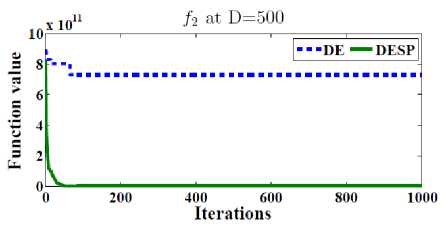
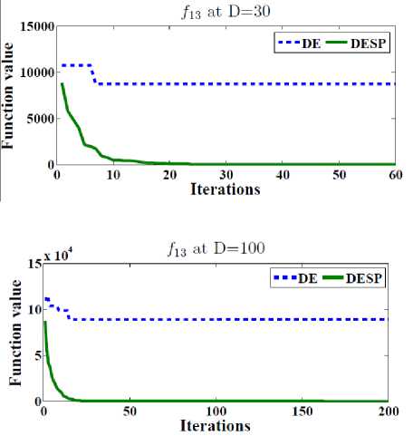
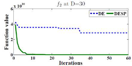
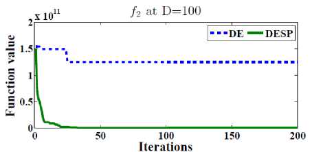
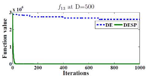
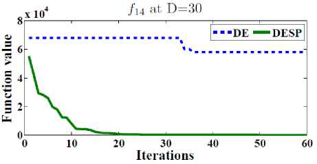
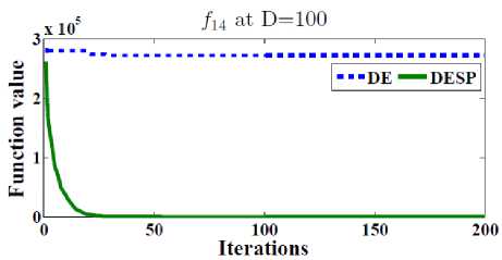
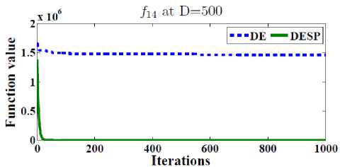
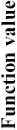
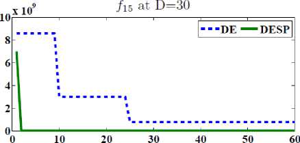
In order to test the efficiency of the space partitioning mechanism, two versions of DESP algorithm (with and without space partitioning) are compared as shown in Figure 2. The dotted line represents the results of DESP without space partitioning while the solid line represents the ones of DESP with space partitioning. Figure 2 gives the general performance of DESP for four of the functions f 2 , f 13 , f 14 and f 15 (randomly picked) with 30, 100, 500 dimensions after 2D iterations. It can be observed that DESP with space partitioning is rapidly converging as the number of generations increases compared to DESP without space partitioning.

scalable on number of dimensions as shown in Table 1. 50 runs were performed for each function. In order to observe the ability to scale up well with the size of the problem, the best, worst, mean, and standard deviations (Std) for D = 10, 30, 100, 200, 500 dimensions are reported in Tables 2. The main termination criterion is the number of iterations is set to 2500 X D.

Iterations

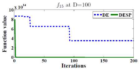
Fig.2. The efficiency of the space partitioning mechanism

2) The General Performance of DESP on Large-Scale Optimization Problems

The efficiency of the space partitioning DESP is tested on 15 benchmark functions. The benchmark functions are

Table 3. Experimental results of DESP for f 1 - f 15 at D=10, 30, 100, 200, 500

D=10
	Best	Worst	Mean		Std
f l	0.0E+00	0.0E+00	0.0E+00		0.0E+00
f 2	4.488E-11	1.75E-09	4.63E-10		8.73E-10
f 3	0.0E+00	2.22E-15	5.18E-16		9.55E-16
f	0.0E+00	7.02E-12	1.88E-12		2.56E-12
f	0.0E+00	1.13E-13	1.61E-14		3.26E-14
f	6.22E-29	1.34E-21	9.08E-21		4.94E-20
f	0.407931	0.407931	4.08E-01		2.82E-16
f a	0.0E+00	0.0E+00	0.0E+00		0.0E+00
f	9.25E-32	1.25E-32	5.24E-32		2.24E-32
^fl0	8.45E-32	5.14E-32	7.58E-32		3.45E-32
f ll	1.84E-53	1.76E-25	1.37E-26		4.54E-26
^fl2	5.77E-13	0.000471	1.57E-05		8.61E-05
^fl3	8.32E-65	6.46E-60	2.51E-61		1.17E-60
f 14	0.00E+0	0.00E+00	0.00E+00		0.00E+00
^fl5	3.6E-177	9.07E-57	3.02E-58		1.65E-57
D=30
f l	0.0E+00	0.0E+00	0.0E+00	0.0E+00
f	4.77E-11	6.96E-11	1.13E-10	1.54E-10
f 3	0.0E+00	0.00E+00	5.18E-16	1.39E-15
f	0.0E+00	9.42E-13	1.01E-11	7.43E-12
f	0.0E+00	0.00E+00	1.19E-13	1.96E-13
f	6.92E-58	3.89E-56	1.03E-09	4.24E-09
f	1.225941	1.225941	1.23E+00	2.25E-16
f a	7.15E-03	5.48E-02	4.89E-02	6.45E-02
f	8.59E-32	5.28E-32	7.56E-32	9.48E-32
^fl0	9.48E-32	3.48E-32	7.58E-32	7.14E-32
f ll	9.11E-26	8.55E-14	2.85E-15	1.56E-14
^fl2	1.92E-10	0.000571	4.84E-05	2.49E-06
^f13	3.00E-63	3.73E-46	1.25E-47	6.81E-47
f 14	0.00E+0	0.00E+00	0.00E+00	0.00E+00
^f15	2.28E-82	3.40E-11	1.13E-12	6.20E-12
D=100
f l	5.32E-23	8.69E-17	2.90E-18	1.58E-17
f 2	8.84E-11	3.21E-05	5.45E-06	1.91E-05
f 3	0.0E+00	2.65E-08	3.84E-09	6.74E-09
f 4	3.44E-11	9.56E-11	5.90E-11	2.20E-11
f₅	0.0E+00	2.16E-12	8.22E-13	6.34E-13
f₆	9.28E-13	6.73E-06	5.34E-07	1.59E-06
f 7	3.111166	3.111166	3.11E+00	1.35E-15
f a	5.48E-01	3.45E+01	4.75E+01	2.79E-02
f 9	8.46E-32	5.24E-32	6.89E-32	5.89E-32
^fl0	7.89E-32	3.82E-32	5.73E-32	4.76E-32
f ll	4.4E-08	3.15E-05	1.13E-06	5.73E-06
^fl2	1.51E-05	0.000865	4.89E-04	7.58E-04
^fl3	3.11E-26	7.74E-10	1.54E-10	1.74E-10
f l4	0.00E+0	0.00E+00	0.00E+00	0.00E+00
^fl5	3.08E-22	2.05E-13	1.63E-14	6.25E-14

D=200
f	2.42E-16	5.16E-15	5.69E-15	1.18E-15
f₇.	1.72E-09	2.77E-02	1.05E-02	0.02557
Л	4.44E-15	8.37E-07	4.24E-08	1.50E-07
f 4	8.27E-12	2.86E-10	8.55E-11	7.38E-11
f	2.13E-04	9.59E-04	0.00064	0.00023
f	9.28E-13	3.29E-04	4.78E-05	8.27E-05
f 7	5.07041	5.07041	5.07E+00	9.03E-16
f	1.78E+01	7.89E+01	4.15E+01	4.78E+01
f	9.78E-32	2.78E-32	4.83E-32	6.59E-32
^f10	4.45E-32	1.67E-32	3.76E-32	5.68E-32
f 11	5.53E-05	0.00022	1.17E-04	6.07E-05
^f12	9.08E-05	0.02431	1.19E-02	5.43E-02
^f13	1.40E-16	9.78E-10	4.39E-10	4.69E-10
f 14	0.00E+00	0.00E+00	0.00E+00	0.00E+00
^f15	3.04E-13	0.004084	1.40E-04	0.000745
D=500
л	4.75E-12	2.73E-11	8.72E-11	5.73E-13
f 2	786.1707	1551.946	1.06E+03	227.0103
f 3	2.22E-10	6.60E-10	3.09E-10	9.08E-11
f 4	3.45E-10	0.0442	3.76E-03	0.011493
f	5.64E-11	0.995	4.97E-01	0.50600
f 6	0.0027	0.186010	1.62E-02	0.037936
f 7	9.0373	9.0373	9.04E+00	1.78E-06
f	5.76E+02	9.73E+02	4.75E+02	5.48E+02
f 9	4.58E-28	5.78E-27	4.73E-28	2.84E-28
^f10	5.76E-29	6.48E-28	1.43E-29	5.48E-29
fn	1.74E-10	2.91E-08	2.20E-09	6.37E-09
^f12	1.28E-06	0.00036	1.43E-05	6.56E-05
/ 13	2.88E-18	5.02E-16	2.06E-17	9.08E-17
f 14	0.00E+00	0.00E+00	0.00E+00	0.00E+00
^f15	1.70E-06	0.00013	2.99E-05	2.43E-05

The results in Tables 2 show that DESP returns a solution with good fitness value within the prescribed number of iterations. For example, DESP obtained mean value equal to zero in three cases for D =10, two cases for D = 30 and one case for D = 100, 200, 500 and lower than 10 ^-6 in ten cases for dimension D = 10, 30, 100 and in six cases for D =200, 500. However, the DESP algorithm seems to encounter some difficulties while optimizing f 2 for D =500, f 7 for D = 30, 100, 200, 500 and f 8 for D = 100, 200 and 500.

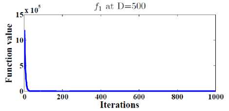
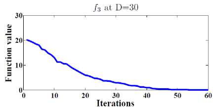
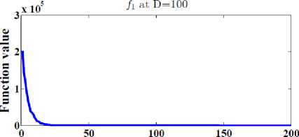
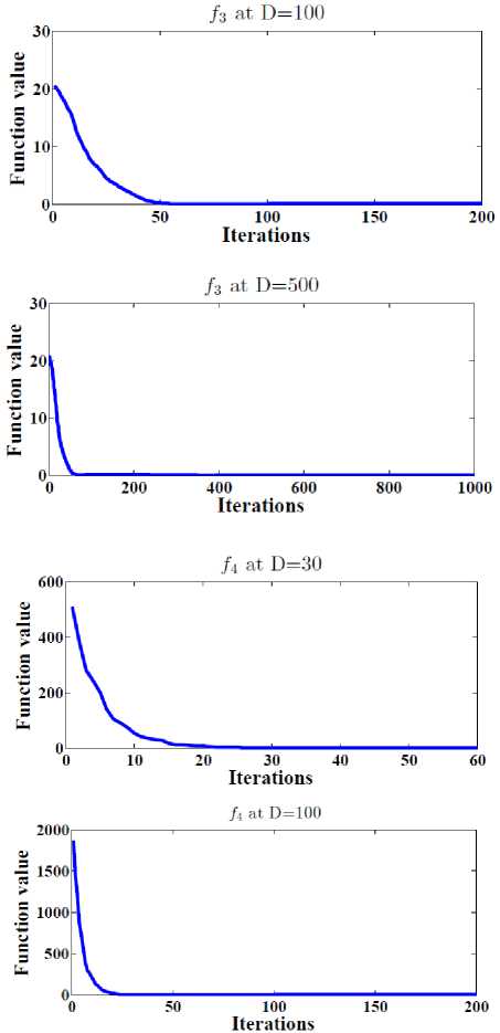
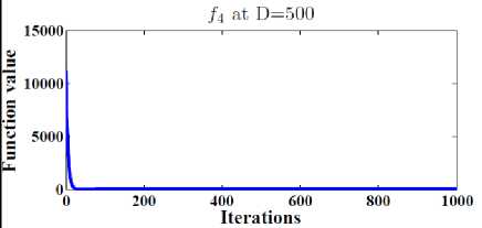
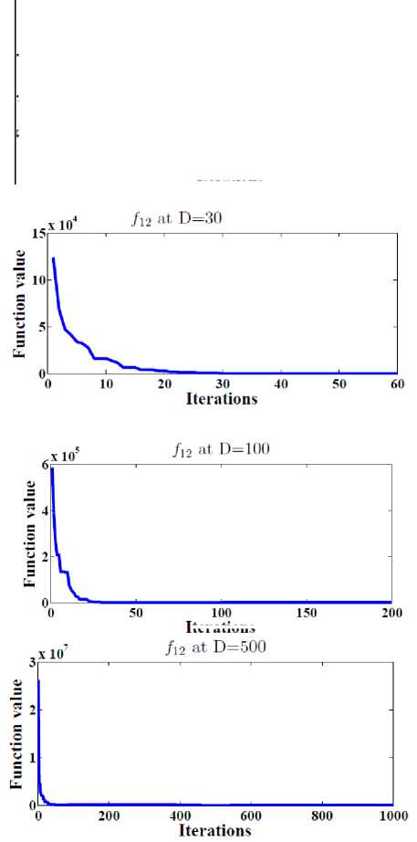
Also, Figure 3 show the general performance of the proposed DESP algorithm by plotting the function values versus the number of iterations after 2D iterations at D= 30, 100, 500 for functions f₁, f₃, f₄, f₁₂ .

We can conclude from Figure 3 that the proposed DESP algorithm can obtain optimal or near optimal solution in a few numbers of iterations.

Iterations

Iterations

Fig.3. The general performance of DESP algorithm

C. DESP Compared Against other Algorithms

The proposed DESP algorithm is tested on ten benchmark functions and compared against three DE algorithms with different mechanisms. The three compared DE algorithms can be described as follow.

• DE (differential evolution). Is the standard differential evolution algorithm [33].
• DEahcSPX (Accelerating differential evolution

using an adaptive local search) [29].

• ADE (An alternative differential evolution

algorithm) [25].

In the following subsection, we highlight the general performance of the proposed algorithm and the other DE algorithms for functions f ₁- f ₁₀ at dimensions 10, 50, 100, 200.

1) DESP Compared to other Algorithms on the Classical

Functions

The general performance of the proposed DESP algorithm is investigated by comparing its results against the results of the other three DE algorithms at dimensions D = 10, 50, 100, 200 for functions f₁-f₁₀ , which are reported in Table 1. In order to make a fair comparison, we have applied the same termination criteria, which the other competitor algorithms are applied. The main termination criterion for all competitor algorithms is chosen as the maximum number of iterations is set to 10000 X D . The population size for the other competitor algorithms was chosen as N = 30 for D = 10 dimensions and for all other dimensions, it was selected as N = D. However, the population size of the proposed DESP algorithm is set to 25. The results of the four competitor algorithms are reported in Tables 4, 5, 6, 7 at dimensions D = 10, 50, 100, 200, respectively. The averaged results (Mean) and the standard deviation (Std) of the function values are reported over 50 independent runs in Tables 4, 5, 6 and 7. The best results are reported in boldface text. The results in Tables 4, 5, 6 and 7 show that the proposed algorithm can obtain the optimal or near optimal solutions in most cases. For example the proposed DESP algorithm results are better than the other competitor algorithms for functions f 1 , f 3 , f 4 , f 5 , f 6 , f 8 ,f 9 ,f 10 at dimension D =10 and for all functions at dimension D =50, 100, 200 except functions f₂, f₉ at dimension D =100 the ADE obtains better values than the proposed algorithm. It is worth to mention that the proposed algorithm is cheaper than the other competitor algorithms due to its number of population size in all cases.

We can conclude form the results in Tables 4, 5, 6 and 7 that the proposed DESP algorithm is a promising algorithm and capable to solve large-scale optimization problems.

Table 4. Comparison of DE, DEahcSPX, ADE and DESP for f1- f10 at D=10 in term of function value

Fun		DE	DEahcSPX	ADE	DESP
A	Mean	3.26E-28	1.81E-38	0.00E+00	0.00E+00
A	Std	5.83E-28	4.94E-38	0.00E+00	0.00E+00
A	Mean	4.78E-01	3.19E-01	1.59E-29	4.48E-11
A	Std	1.32E+00	1.10E+0	2.61E-29	1.75E-09
A	Mean	8.35E-15	2.66E-15	5.32E-16	0.00E+00
A	Std	8.52E-15	0.00E+00	1.77E-15	0.00E+00
A	Mean	5.75E-02	4.77E-02	4.43E-4	0.00E+00
A	Std	3.35E-02	2.55E-02	1.77E-03	0.00E+00
^A	Mean	1.85E+00	1.60E+00	0.00E+00	0.00E+00
^A	Std	1.68E+00	1.61E+00	0.00E+00	0.00E+00
A	Mean	14.2127	4.7376	0.00E+00	0.00E+00
A	Std	39.2815	23.6876	0.00E+00	0.00E+00
A	Mean	0.1078	0.0998	0.0998	9.03E-03
A	Std	0.0276	3.47E-08	7.60E-12	5.12E-10
A	Mean	18.1122	18.0069	0.00E+00	0.00E+00
A	Std	15.8578	13.1127	0.00E+00	0.00E+00
A	Mean	3.85E-29	4.71E-32	4.71E-32	9.23E-32
A	Std	7.28E-29	1.12E-47	1.11E-47	2.25E-47
/ 10	Mean	1.49E-28	1.35E-32	1.34E-32	3.25E-32
/ 10	Std	2.20E-28	5.59E-48	1.10E-47	4.15E-47

Table 5. Comparison of DE, DEahcSPX, ADE and DESP for f1- f10 at D=50 in term of function value

Fun		DE	DEahcSPX	ADE	DESP
/	Mean	5.91E-02	8.80E-09	6.40E-94	0.00E+00
/	Std	9.75E-02	2.80E-08	2.94E-93	0.00E+00
A	Mean	1.13E+10	1.63E+02	9.27E-06	6.34E-11
A	Std	2.34E+10	3.02E+02	2.00E-05	2.32E-09
/ з	Mean	2.39E-02	1.69E-05	5.15E-15	0.00E+00
/ з	Std	8.90E-03	8.86E-06	1.64E-15	0.00E+00
/ 4	Mean	7.55E-02	2.96E-03	0.00E+00	0.00E+00
/ 4	Std	1.14E-01	5.64E-03	0.00E+00	0.00E+00
Л	Mean	6.68E+01	3.47E+01	0.00E+00	0.00E+00
Л	Std	2.36E+01	9.23E+00	0.00E+00	0.00E+00
A,	Mean	1.07E+03	9.56E+02	0.00E+00	0.00E+00
A,	Std	5.15E+02	2.88E+02	0.00E+00	0.00E+00
/ 7	Mean	1.15E+00	4.00E-01	2.27E-01	1.25E-02
/ 7	Std	1.49E-01	1.00E-01	4.53E-02	5.24E-01
/ 8	Mean	1.43E+05	1.41E+03	3.01E+02	9.25E+01
/ 8	Std	4.10E+05	2.90E+02	2.12E+02	3.25E+01
/ ,	Mean	3.07E-02	2.49E-03	1.42 E-32	4.25E-32
/ ,	Std	7.93E-02	1.24E-02	1.35E-32	3.78E-32
^/10	Mean	2.24E-01	2.64E-03	4.85E-32	9.25E-32
^/10	Std	3.35E-01	4.79E-03	5.57E-32	6.14E-32

Table 7. Comparison of DE, DEahcSPX, ADE and DESP for f1- f10 at D=200 in term of function value

Fun		DE	DEahcSPX	ADE	DESP
/ 1	Mean	1.26E+05	7.01E+03	4.28E-22	1.45E-35
/ 1	Std	1.06E+04	1.07E+03	4.50E-22	2.45E-35
/ 2	Mean	2.97E+10	1.11E+08	2.33E+02	1.72E-09
/ 2	Std	3.81E+09	2.63E+07	2.52E+01	2.77E-02
/ 3	Mean	1.81E+01	8.45E+00	7.12E-13	4.44E-15
/ 3	Std	2.26E-01	4.13E-01	3.44E-13	8.37E-14
/ 4	Mean	1.15E+03	6.08E+01	2.37E-16	8.27E-16
/ 4	Std	9.22E+01	9.30E+00	2.03E-16	2.86E-16
/ 5	Mean	2.37E+03	1.53E+03	1.03E+01	9.59E-04
/ 5	Std	7.24E+01	8.31E+01	3.59E+00	2.13E-04
/ 6	Mean	6.66E+04	6.61E+04	0.00E+00	0.00E+00
/ 6	Std	1.32E+03	1.44E+03	0.00E+00	0.00E+00
/ 7	Mean	3.69E+01	1.10E+01	4.33E-01	3.58E-02
/ 7	Std	1.80E+00	4.38E-01	4.78E-02	4.59E-02
/ 8	Mean	3.13E+18	4.21E+13	1.26E+03	1.58E+01
/ 8	Std	9.48E+17	1.74E+13	8.07E+02	2.58E+01
/ ,	Mean	3.49E+08	2.27E+01	1.31E-20	5.48E-32
/ ,	Std	7.60E+07	5.73E+00	2.83E-20	4.89E-32
/ 10	Mean	8.08E+08	6.24E+04	1.31E-20	9.84E-31
/ 10	Std	1.86E+08	4.77E+04	1.36E-20	5.48E-32

Table 6. Comparison of DE, DEahcSPX, ADE and DESP for f1- f10 at D=100 in term of function value

Fun		DE	DEahcSPX	ADE	DESP
/ 1	Mean	4.28E+03	5.01E+01	6.37E-45	5.32E-35
/ 1	Std	1.27E+03	8.94E+01	1.12E-44	8.69E-27
/ 2	Mean	3.33E+08	1.45E+05	8.90E+01	8.84E-11
/ 2	Std	1.67E+08	1.11E+05	3.46E+01	3.21E-05
/	Mean	8.81E+00	1.91E+00	6.21E-015	0.00E+00
/	Std	8.07E-01	3.44E-01	0.00E+00	0.00E+00
/ 4	Mean	3.94E+01	1.23E+00	0.00E+00	0.00E+00
/ 4	Std	8.01E+00	2.14E-01	0.00E+00	0.00E+00
^f 5	Mean	8.30E+02	4.75E+02	0.00E+00	0.00E+00
^f 5	Std	6.51E+01	6.55E+01	0.00E+00	0.00E+00
A,	Mean	2.54E+04	2.48E+04	0.00E+00	0.00E+00
A,	Std	2.15E+03	2.14E+03	0.00E+00	0.00E+00
/ 7	Mean	1.02E+01	3.11E+00	3.03E-01	7.34E-02
/ 7	Std	7.91E-01	5.79E-01	1.97E-02	4.13E-01
/ 8	Mean	5.44E+15	4.06E+10	7.70E+02	4.75E+01
/ 8	Std	5.07E+15	6.57E+10	8.69E+02	6.14E+01
/ ,	Mean	6.20E+05	4.34E+00	9.18E-33	7.25E-33
/ ,	Std	7.38E+05	1.75E+00	8.09E-33	5.47E-33
^/10	Mean	4.34E+06	7.25E+01	6.40E-32	8.14E-32
^/10	Std	2.30E+06	2.44E+01	5.87E-32	6.58E-32

VI. Conclusion

A new DE algorithm has been proposed in this paper in order to solve large-scale global optimization problems. The proposed algorithm is called deferential evolution with space partitioning (DESP). The use of space variable partitioning effectively assists the proposed algorithm to explore the search space and accelerate the search. The partitioning mechanism works as dimensional reduction mechanism. The proposed algorithm has been applied on different classical benchmark functions and compared against three variant DE algorithms. The numerical resuluts show that the proposed algorithm is a promising algorithm and it is cheaper than the other DE algorithms and can obtain the optimal or near optimal solution for large-scale optimization problems in reasonable time.

Список литературы Differential Evolution Algorithm with Space Partitioning for Large-Scale Optimization Problems

A.F. Ali, A. E. Hassanien, V. Sná?el, and M. F. Tolba, “A New Hybrid Particle Swarm Optimization with Variable Neighborhood Search for Solving Unconstrained Global Optimization Problems,” Advances in Intelligent Systems and Computing, pp. 151–160, 2014.
A.F. Ali, “Hybrid Simulated Annealing and Nelder-Mead Algorithm for Solving Large-Scale Global Optimization Problems”. International Journal of Research in Computer Science, 4 (3): pp. 1-11, May 2014.
J. Brest, MS. Maucec Population size reduction for the differential evolution algorithm. Appl Intell, 29:228–247, 2008
S.A. Chu, P.-W. Tsai, and J.-S. Pan. Cat swarm optimization. Lecture Notes in Computer Science (including subseries Lecture Notes in Arti_cial Intelligence and Lecture Notes in Bioinformatics), 4099 LNAI:854-858, 2006.
S. Das, A. Abraham, UK. Chakraborty, A. Konar Differential evolution using a neighborhood-based mutation operator. IEEE Trans Evol Comput, 13(3):526–553, 2009.
M. Dorigo, Optimization, Learning and Natural Algorithms, Ph.D. Thesis, Politecnico di Milano, Italy, 1992.
A. Duarte, R. RMarti, F. Glover, F. Gortazar, Hybrid scatter tabu search for unconstrained global optimization. Ann Oper Res 183:95–123, 2011.
N. Hansen, The CMA evolution strategy: a comparing review. In: Lozano JA, Larra?aga P, Inza I, Bengoetxea E(eds) Towards a new evolutionary computation. Springer, Berlin, 2006.
P. Hansen, N. Mladenovic, JA. Pérez Variable neighbourhood search: methods and applications. Ann Oper Res 175(1):367–407, Moreno, 2010.
A. Hedar and A.F. Ali, Tabu Search with Multi-Level Neighborhood Structures for High Dimensional Problems Applied Intelligence, Springer, 2012.
A. Hedar, A. Fouad, Genetic algorithm with population partitioning and space reduction for high dimensional problems. In: Proceeding of the 2009 international conference on computer engineering and systems (ICCES09), Cairo, Egypt, pp 151–156, 2009.
A. Hedar, M. Fukushima, Hybrid simulated annealing and direct search method for nonlinear unconstrained global optimization. Optim Methods Softw 17:891–912, 2002.
F. Herrera, M. Lozano, JL. Verdegay, Tackling real-coded genetic algorithms: Operators and tools for behavioral analysis. Artif Intell Rev 12:265–319, 1998.
F. Herrera, M. Lozano, D. Molina, Continuous scatter search: An analysis of the integration of some combination methods and improvement strategies. Eur J Oper Res 169(2):450–476, 2006.
D. Karaboga and B. Basturk. A powerful and efficient algorithm for numerical function optimization: artificial bee colony (abc) algorithm. Journal of global optimization, 39(3):459-471, 2007.
J. Kennedy, RC. Eberhart, Particle Swarm Optimization, Proceedings of the IEEE International Conference on Neural Networks, Vol 4, pp 1942-1948, 1995.
M. Laguna, R. Martí, Experimental testing of advanced scatter search designs for global optimization of multimodal functions. J Glob Optim 33(2):235–255, 2005.
CY. Lee, X. Yao, Evolutionary programming using the mutations based on the Lévy probability distribution. IEEE Trans Evol Comput 8:1–13, 2004.
YW. Leung, Y. Wang, An orthogonal genetic algorithm with quantization for global numerical optimization. IEEE Trans Evol Comput 5(1):41–53, 2001.
M. Lozano, F. Herrera, N. Krasnogor, D. Molina, Real-coded memetic algorithms with crossover hill-climbing. Evol Comput 12(3):273–302, 2004.
X.L. Li, Z.J. Shao, and J.X. Qian. Optimizing method based on autonomous animats: Fish-swarm algorithm. Xitong Gongcheng Lilun yu Shijian/System Engineering Theory and Practice, 22(11):32, 2002.
JJ. Liang, AK. Qin, PN. Suganthan, S. Baskar Comprehensive learning particle swarm optimizer for global optimization of multimodal functions. IEEE Trans Evol Comput 10(3):281–295, 2006.
Y. Li, X. Zeng, Multi-population co-genetic algorithm with double chain-like agents structure for parallel global numerical optimization. Appl Intell 32:292–310, 2010.
M.H. Mashinchia, MA. Orguna, W. Pedryczb, Hybrid optimization with improved tabu search. Appl Soft Comput 11(2):1993–2006, 2011.
A.W. Mohamed, H.Z. Sabry and M. Khorshid, An alternative differential evolution algorithm for global optimization, Journal of advanced research, 3, 149-165, 2012.
N. Mladenovic, M. Drazic, V. Kovac, M. Angalovic General variable neighborhood search for the continuous optimization. Eur J Oper Res 191:753–770, 2008.
H. Mühlenbein, D. Schlierkamp, Predictive models for the breeder genetic algorithm. IEEE Trans Evol Comput 1(1):25–, 1993.
QH. Nguyen, YS. Ong, MH, Lim, A probabilistic memetic framework. IEEE Trans Evol Comput 13(3):604–623, 2009.
N. Noman, H. Iba, Accelerating differential evolution using an adaptive local search. IEEE Trans Evol Comput 12(1):107–125, 2008.
ZJ. Pan, LS. Kang, An adaptive evolutionary algorithms for numerical optimization. In: Yao X, Kim JH, Furuhashi T (eds) Simulated evolutionary and learning. Lecture notes in artificial intelligence. Springer, Berlin, pp 27–34, 1997.
M.K. Passino, Biomimicry of bacterial foraging for distributed optimization and control. Control Systems, IEEE 22(3):52-67, 2002.
KV. Price, RM. Storn, JA. Lampinen, Differential evolution: a practical approach to global optimization. Springer, Berlin, 2005.
R. Storn, K. Price, Differential evolution a simple and efficient heuristic for global optimization over continuous spaces. J Glob Optim 11:341-359, 1997.
K. Socha, M. Dorigo, Ant colony optimization for continuous domains. Eur J Oper Res 185(3):1155–1173, 2008.
R. Tang, S. Fong, X.S. Yang, and S. Deb. Wolf search algorithm with ephemeral memory. In Digital Information Management (ICDIM), 2012 Seventh International Conference on Digital Information Management, pages 165-172, 2012.
D. Teodorovic and M. DellOrco. Bee colony optimizationa cooperative learning approach to complex tranportation problems. In Advanced OR and AI Methods in Transportation: Proceedings of 16th MiniEURO Conference and 10th Meeting of EWGT (13-16 September 2005).Poznan: Publishing House of the Polish Operational and System Research, pages 51-60, 2005.
AK. Qin, VL. Huang, PN. Suganthan, Differential evolution algorithm with strategy adaptation for global numerical optimization. IEEE Trans Evol Comput 13(2):298–417, 2009.
JA. Vrugt, BA. Robinson, JM. Hyman, Self-adaptive multimethod search for global optimization in real-parameter spaces. IEEE Trans Evol Comput 13(2), 2009.
X.S. Yang. A new meta-heuristic bat-inspired algorithm. Nature Inspired Cooperative Strategies for Optimization (NICSO 2010), pages 6574, 2010.
X.S. Yang. Firey algorithm, stochastic test functions and design optimisation. International Journal of Bio-Inspired Computation, 2(2):78-84, 2010.
X. Yao, Y. Liu, G. Lin, Evolutionary programming made faster. IEEE Trans Evol Comput 3(2):82–102, 1999.
W. Zhong, J. Liu, M. Xue, L. Jiao, A Multiagent genetic algorithm for global numerical optimization. IEEE Trans Syst Man Cybern, Part B, Cybern 34(2):1128–1141, 2004.

Еще

Статья научная

Differential Evolution Algorithm with Space Partitioning for Large-Scale Optimization Problems

Текст научной статьи Differential Evolution Algorithm with Space Partitioning for Large-Scale Optimization Problems

IV. Differential Evolution with Space Partitioning (Desp)

7: repeat

V. Numerical Experiments

VI. Conclusion

Список литературы Differential Evolution Algorithm with Space Partitioning for Large-Scale Optimization Problems