Fundamentals of calculation of random vibration acceleration signals during high-speed track tests of new aircraft samples

The fundamentals of calculating the responses of mechanical systems subject to external random disturbances are based on the general principles of vibration and impact theory. In the practice of studying vibration characteristics, the dynamics of aircraft motion are often represented by the relationship between the spectral density of an ergodic process and the Fourier transform of specific realizations of a random process, which are non-periodic functions over a certain time interval and assumed to be zero outside this interval. The methodology for calculating the responses of elastic structural elements of track carriages is based on the theory of random processes [1–4], the fundamentals of vibration theory [5–7], and the practice of applying experimental data processing [8–15]. A comparative analysis with test data in foreign studies [16–20] has been conducted. For random processes, an estimate of the probability of the distribution of signals from vibration and impact external influences on the structural element under consideration is used. With several experiments, the relative frequency of occurrence of event values tends to unity, depending on the number of measurements. However, the conditions that characterize real high-speed track tests and the assumptions about the quasi-stationarity of processes in these cases, and especially the ergodicity of random vibration of structural elements, are often inconsistent. As track carriages accelerate, the vibration acceleration amplitudes along the X, Y, and Z axes increase with varying regularities. Here, the moving X coordinate coincides with the direction of motion, the Y axis points vertically upward, and the Z coordinate reflects lateral displacements.

Objectives and tasks of the work

The aim of this work is to investigate the influence of the monorail experimental setup (ED) on the vibration of a test article during acceleration from transonic speeds to the establishment of a supersonic shock wave system. The objectives of the work include increasing the reliability of the obtained experimental values by refining the values of random vibration accelerations of the reaction of structural elements during significantly non-stationary acceleration during track tests of articles on the "Rocket Rail Track 2500" facility of the L.K. Safronov State Research Institute of Aerospace Engineering. The experimental data were processed using Fourier transforms and wavelet decomposition.

The article systematizes the principles of analysis of random vibration acceleration signals obtained by autonomous vibration acceleration sensors – recorders placed in the carriage shoes and the test object simulator.

General provisions for assessing random vibrations under non-stationary loading

During high-speed track testing, the elements of track carriages and the test articles are subject to external influences of a random nature. Between the sensor readings and the sought statistics of spectral densities or correlation functions, an evidentiary basis for the applicability of known principles on which the method for calculating the structural response is based must be presented. The response of a structure to random pulses whose distributions obey the normal law also has a normal distribution for linear and near-linear systems [1–4; 8–10]. Determining the correlation function, and accordingly the spectral density of the response of structural elements, from the recordings of vibration acceleration signals from sensors is sufficient to describe a random process with a normal distribution. For linear systems, the principle of superposition is observed, i.e., the addition of the responses of a large number of independent processes with a distribution of values close to a Gaussian dependence. Considering the short duration of non-periodic impacts and their relatively low energy, we assume the validity of Hooke's law under vibro-impact loading of structural elements. On the other hand, we bear in mind that there are a sufficient number of factors influencing the formation of errors in the readings of autonomous sensors of the BC 327 type, which have high sensitivity and low temporal inertia. In the case of a non-stationary random process, it is difficult to isolate a time range with the assumption of quasistationarity of the stochastic implementation for describing the statistics. Within the framework of the time intervals under consideration, we will apply well-known approaches with the Fourier transform, but, unlike them, we will determine the statistics only for the maximum impacts. In this case, we assume that the input impacts { X ( t )} have average values m X ( t ) = E [ x ( t ) ] , and their correlation function K X ( t , t +τ) can be determined in this time interval using the dependencies adopted in [3].

Let us consider the response of a sensor placed in a test object simulator m _to . We will isolate the vertical coordinate y and assume the linearity of the system for the particular case considered in the article. Under external vibration and impact influences, the structural elements of the carriage are subject to linear deformations within the limits of Hooke's law. In this case, the mechanical linear system acts as a shaping filter for the spectral density of the signal output in a narrow frequency band. Vibratory mechanical systems without dampers are weakly damped, and the responses of such structures to external random influences f e _ri ( t ) are narrow-band random Gaussian processes with zero mean value [1; 2]. In this case, the implementation of random signals of vertically directed vibration accelerations of the sensor placed in the test object simulator can be represented by sinusoidal oscillations with randomly varying amplitude and phase:

m to y + P f y + ky = f en ( t ) ,                                    ⁽¹⁾

where k is system rigidity; « 2, = k / m _to is natural frequency of the test object simulator; p _f is vibration damping coefficient.

Considering the following conditions, that when t > tо У (t0 ) = a; y (tо ) = b.                                         (2)

Let us denote the damping coefficient as ς and transform formula (3) taking into account

P f / m to = ²W ^f tri ( t ) / ^m to = z ( t ) , to the next view for t >  t 0

y + 2®0^У + ю° У = z (t), the reaction of the system can be represented as follows [1; 2]

t y ( t ) = ay 1 ( t - 1 ₀ ) + by ₂ ( t - 1 ₀ ) + j h ( t - t ) z ( t ) d t , t ₀

where h ( t -t ) is impulse function.

In this case, the response of a linear system to a random input can be written as the sum of the following components y1 (t) = e-?“°t {cosюt + -^0-sinюt];                                 (6)

\ ю 7

where ю = ю0 1 -g2, y2 (t ) = h (t ) = 4 e<ю"t sin юt,                                     (7)

ю for values 0 < g < 1.

In the case of weak damping, the mathematical expectation of the stochastic process can be written taking into account conditions (2)

t mY (t) = ay1 (t -1°) + by 2 (t -1°) +j h (t -t)mY (t) dt,                       (8)

t ₀

then the correlation function of the output signal will look like

K YY ( t 1 , t 2 ) = E [ y ( t 1 ) ^- m Y ( t 1 ) ][ y ( t 2 ) ^- m Y ( t 2 ) ] = ^{t 1 t 2}                                                                                             (9)

= j d ^t 1 + j h ( t 1 ^-t 1 ) h ( t 2 ^-t 2 ) K YY ( ^t 1, ^t 2 ) d ^t 2 .

t ₀ t ₀

Similarly, the dispersion can be expressed by substituting the expression into formula (9) t 1 = t 2 = t .

Following the Wiener-Khinchin generalizations given in [3; 8], the response of linear systems with infinite time of action to non-stationary input effects can be represented through an impulse response function and the application of Fourier transforms in the form

«

Y ( f ) = j h ( t ) e ^- j ^{2 n ft} dt ,                                        (10)

-« here ю = 2nf.

In a simplified form, the time-averaged values of the squared response for the spectral density of signals of a weakly damped system with a filter property can be represented by the dependence [4; 10; 21; 22]

S 0 = ² c(_nE Г y ² ( t ) ] . n

Evaluation of the dynamic state of the structure of the tested product based on the readings of vibration acceleration sensors

Let us consider the state of the payload simulator when adding up the effects in the vertical direction from the aerodynamic drag forces and the moments from their applications, as well as the vibrations transmitted from the front shoe of the track carriage.

The state of the sensor during carriage movement along the X -axis is characterized by the simultaneous vertical displacement of the front shoe coordinate y b ( t ), the velocity of movement being y _b ( t ) , and the acceleration being y _b ( t ) . We denote the vertical displacement of the sensor as y _s ( t ) , and the velocity as y _s ( t ) , and the acceleration as y = y _s ( t ) - y _b ( t ) . We introduce a new variable for vertical displacement in the form, and represent the equation for the oscillations of the mass of the test article m to in the vertical plane:

m to ( ^y + ^y b ) + P f ^{y +} ky = 0, ⁽¹²⁾

where k is system rigidity; ( 2 = k / m _to - natural frequency of the test object simulator; P _f is vibration damping coefficient.

Let us introduce the relative value of the loss coefficient through the ratio to the critical value

Pf

C = —f— and denote the relationship in the following form 2ю0^ = Pf / mto. Then dependence (12) Pf _cr can be divided with respect to the variable displacements of the front shoe and the displacements of the test object simulator.

Index of the friction loss coefficient β f_cr means the critical value of the vibration damping coefficient.

^y + ^q y I (% y = - ^y b .                              ⁽¹³⁾

To determine the transfer function of the test object simulator, we introduce a disturbance in the form of a pulse transmitted from the front shoe with the index designation – b_1

( -и ² + j 2 c((_N + ( ) y i e^J “ t = - y b! e^J “ t ,

here j is imaginary quantity; ω is forced oscillation frequency.

Transfer function H• (®), reflecting the dynamic connection between the front shoe and the test object simulator, will take the form

Hi (®) =

y ₁

• • yb_1

-1

2    (      (

(0 1 - —2 + J 2c

I (0      (0 J

We assume that the spectral density of the disturbance is S 1 ( и ) in the range of the sensor filter bandwidth for the response at the resonance frequency ® = ® ₀ is approximately constant, then the root mean square value of the response r ² can be determined from the expression (11) [7–10]

r ² = j H ( _ю)| ² S 1 ( a ) d _ю .

The spectral density of the acceleration of the front shoe S y b ( ю ₀ ) (or the base of the track carriage) is used to determine the root-mean-square value of the reaction of vertical vibration displacements recorded by the sensor,

У b² =

S y b ^(w 0 ) ^ю 0

j

V 0

1 -

d ю

ю I

1^Ю 0

+ 2^| l юо J

where ς is damping coefficient of the system.

Taking into account relationships (7)–(11), we present the processing of random signals from a fullscale experiment. We demonstrate that the distribution of random variables follows the normal distribution law or is reasonably close to it. For example, to assess the stresses in the carriage elements' structure, with large deviations from the mean ^ = y - m_y ( t ) , we estimate the probability that the stresses do not exceed permissible values.

Description of the experiment and results of vibration acceleration processing

Let us estimate the contribution of vibration accelerations measured by sensor No. 2, located in the front shoe, transmitted through the structure of the front bracket to the test object (Fig. 1).

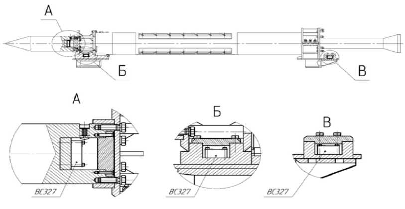
Рис. 1. Конструктивная схема размещения датчиков виброускорений ВС 327:

А – имитатор объекта испытания с внутренней нишей для датчика № 1; Б – передний башмак (опора скольжения) с отсеком для размещения датчика № 2; В – задний башмак с контейнером для датчика № 3

Fig. 1. Structural diagram of the placement of vibration acceleration sensors VS 327:

A – test object simulator with an internal niche for sensor No. 1; Б – front shoe (sliding support)

with a compartment for sensor No. 2; B – rear shoe with a container for sensor No. 3

Let us consider the response of the sensitive element of the three-axis vibration acceleration sensor No. 1 type BC 327, placed inside the payload simulator during high-speed track tests [15–16] (Fig. 2).

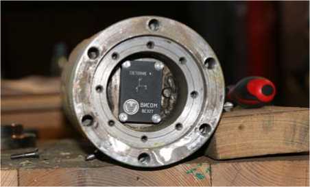
Рис. 2. Фотография размещения датчика ВС 327 в полости имитатора объекта испытания

Fig. 2. Photograph of the placement of the BC 327 sensor in the cavity of the test object simulator

The sensor housing is rigidly connected to the test object simulator; their combined mass is m to = 50 kg. The simulator's mass is assumed to be concentrated, and the test object simulator itself is cantilevered. The test object center of mass is located on the carriage axis and offset by a distance l 1 relative to the mounting in the front bracket.

The distance from the mounting to the center of mass of sensor № 1 is l 2 , which is also located on the axis of the test object simulator. We assume that the mass of the sensor's elastic element is small compared to the mass of the rigid body m to . We represent the calculation model as an elastic cantilever beam with a concentrated load at the center of mass of the test object simulator. We denote: E is Young's modulus, I is the moment of inertia of the cross-sectional area.

Beam deflection δ y at the center of mass will be [7]

If we substitute the acting force F ( t ) into the right side of equation (1) and carry out similar transformations, then instead of vibration displacements we can obtain a ratio similar to formula (18) for the square of the average value of displacement near the resonant frequency for the test object simulator in the form

—2             ПГО о

y ~ S F/k ^(w 0 )~.   .

4^

Here S _F/k ( w ) is spectral density of vibration displacements in the direction of the axis Y .

For the case of low system damping at frequencies near natural resonances, the vibration modes are close to those of an undamped beam. The free vibration equation for the transverse deflection of a conventionally homogeneous beam can be written as [1; 3; 4; 7; 9; 11; 13–15]

dX + m- dX = 0 dx4 11 ei d t2      .

The known solution for this equation for small displacements is от

k = 1

Here ф _k ( x ) is natural vibration modes with natural frequency ю n _k , and £ k ( t ) is intensity of the oscillation mode over time.

Natural modes for the case of a homogeneous beam are determined using Krylov's coefficients [7]. Expressions for free modes of vibration and frequency equations for various boundary conditions are presented in [7; 13–15], as well as tables of numerical values of vibration modes and their derivatives. In the case under consideration, we will limit ourselves to the first mode of beam bending. We assume that the maximum stress is directly proportional to the bending moment in the section under consideration, multiplied by the beam thickness and divided by twice the moment of inertia of the crosssectional area.

Fig. 3 shows a graph of the vibration acceleration signal of sensor № 1 in the direction of the vertical Y axis located inside the test object simulator.

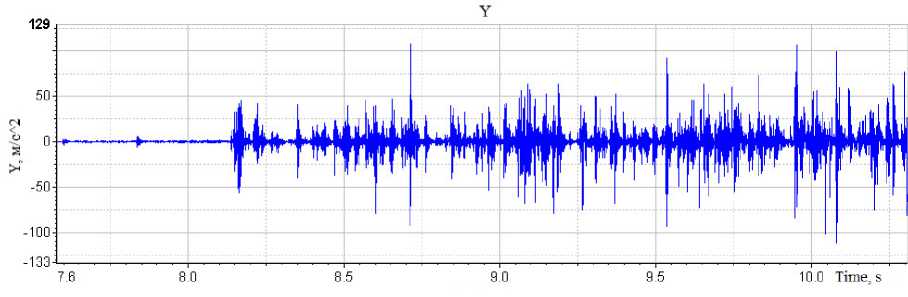
Рис. 3. График виброускорений датчика № 1 по направлению вертикальной оси Y за время движения экспериментальной установки от t 0 = 7,8 с до t 1 = 10,5 с на начальном участке разгона до скорости V = 423 м/с. Пуск ЭУ 20.09.2024 г.

Fig. 3. Graph of vibration accelerations of sensor No. 1 in the direction of the vertical Y axis during the movement of the experimental setup from t 0 = 7.8 s to t 1 = 10.5 s during the acceleration section to a speed of V = 423 m/s. Experimental rocket sled start-up on September 20, 2024

The ordinate axis shows the vibration acceleration values in m/s2, and the abscissa axis shows the time in seconds, tied to the moving coordinate system.

A distinctive feature of the experimental setup motion dynamics is the response of the test object simulator to individual impacts, the amplitudes of which exceed the average level of vertically directed vibration accelerations by 3–5 times. The values of the maximum vertical vibration accelerations shown in this graph are equal to А Y = +107.015 m/s², realized at the time t = 8.71371 s at the carriage speed V = 148 m/s. The maximum negative amplitude values are equal to А Y = –120.455 m/s², they were realized at the time t = 10.32269 s at the supersonic speed V = 403 m/s. The signal processing and its spectral characteristics are performed on the basis of Fourier transforms [11; 21–27].

Fig. 4 shows an image of the autocorrelation function (ACF) of the signal of vertically directed vibration accelerations of sensor No. 1.

The ACF plot of the vibration accelerations of sensor № 1 along the vertical Y -axis displays a weakly damped sum signal of random vibration accelerations (see formula (9)). The ACF modulus reaches zero after 1.6 c.u.; after this point, the noise components of the signal disappear. The autocorrelation function displays the sum of several harmonic signals with a variable period or a complex qu-asi-periodic sum signal. Figure 5 shows the probability density distribution plot of random vertical vibration acceleration signals of sensor № 1, located in the test object simulator.

The ACF plot of the vibration accelerations of sensor № 1 along the vertical Y-axis displays a weakly damped sum signal of random vibration accelerations (see formula (9)). The ACF modulus reaches zero after 1.6 c.u.; after this point, the noise components of the signal disappear. The autocorrelation function displays the sum of several harmonic signals with a variable period or a complex qu-asi-periodic sum signal. Figure 5 shows the probability density distribution plot of random vertical vibration acceleration signals of sensor № 1, located in the test object simulator. The ACF plot of the vibration accelerations of sensor № 1 along the vertical Y-axis displays a weakly damped sum signal of random vibration accelerations (see formula (9)). The ACF modulus reaches zero after 1.6 c.u.; after this point, the noise components of the signal disappear. The autocorrelation function displays the sum of several harmonic signals with a variable period or a complex quasi-periodic sum signal. Figure 5 shows the probability density distribution plot of random vertical vibration acceleration signals of sensor № 1, located in the test object simulator.

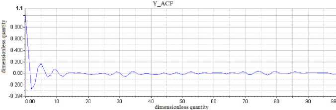
Рис. 4. График автокорреляционной функции виброускорений датчика № 1 по направлению вертикальной оси Y за время движения ЭУ от t 0 = 7,8 с до t 1 = 10,5 с на участке разгона

Fig. 4. Graph of the autocorrelation function of vibration accelerations of sensor No. 1 in the direction of the vertical Y axis during the movement of the experimental rocket sled from t 0 = 7.8 s to t 1 = 10.5 s in the acceleration section

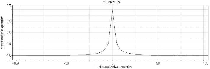
Рис. 5. График одномерной плотности вероятности случайного процесса пиковых значений датчика № 1 по направлению вертикальной оси Y за время движения от t 0 = 7,8 c до t 1 = 10,5 c ЭУ на участке разгона

Fig. 5. Graph of the one-dimensional probability density function of the random process of peak values of sensor No. 1 in the direction of the vertical Y axis during the movement of the experimental rocket sled from t 0 = 7.8 s to t 1 = 10.5 s in the acceleration section

The probability distribution graph for peak values in a narrowband process is close to the Rayleigh distribution law. For oscillatory systems with sharp resonances and in the case of exciting oscillations representing Gaussian white noise, the mathematical expectation of the frequency coincides with the natural frequency of the system [1; 9; 10]. The system's response to a narrowband random process corresponds to the root-mean-square value of the structure's response to the action of a harmonic. To the simultaneous action of several narrowband random processes, the oscillatory system responds as to polyharmonic vibrations. The variance is less than 9 %, but there is asymmetry in the distribution and significant excess (peakedness of the distribution). Knowing the permissible stress specified in the technical specifications (TS), it is possible to determine the permissible disturbance value such that the probability of exceeding it is sufficiently low. The probability of exceeding the limit value of displacements during a certain fraction of the total time can be calcul ated i f we take for the displacement of the i -th harmonic under the normal distribution law, then n^ = _л Ila? .

ix ix

Index x is the current value of the ensemble of random vibration acceleration variables.

This consideration is natural for any form of vibration of a real structure.

Fig. 6 shows a graph of vibration displacements for vertical signals from sensor № 1 before the front shoe breaks contact with the upper surface of the rail head.

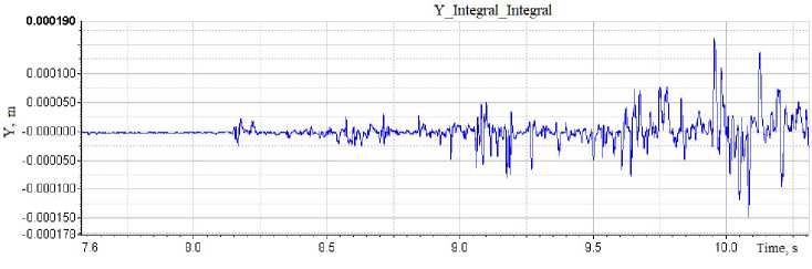
Рис. 6. График виброперемещений случайного процесса пиковых значений датчика № 1 по направлению вертикальной оси Y на участке разгона экспериментальной установки до скорости V = 423 м/с. Пуск ЭУ 20.09.2024 г.

Fig. 6. Graph of vibration displacements of the random process of peak values of sensor No. 1 in the direction of the vertical Y-axis during the acceleration of the experimental setup to a speed of V = 423 m/s. The power plant was launched on September 20, 2024

In Fig. 1, the vertical ordinate axis is measured in meters. The vibration displacement amplitude graphs are ±-directed relative to zero. This characterizes the vertical displacement of the sensor mounted on a cantilevered beam. During the acceleration section, the vertical vibration displacements recorded by sensor № 1 are insignificant. However, it should be noted that sensor № 1 is located near the end-piece (cantilever rod) of the test object simulator at a distance of l 2 = 0.08 m, while the rod's center of mass is shifted forward by a distance of l 1 = 0.2 m relative to the end-piece. Otherwise, the displacements of the test object's center of mass will be 2.5 times greater than the values obtained from sensor № 1. The vertical displacements of the test object simulator are determined by the following components: on the one hand, the vertical displacements of the front shoe, which is structurally connected to the front bracket and contacts the rail, which has vertical deviations from straightness (the displacements are limited by the vertical gap between the contact surfaces of the shoe and the railhead); on the other hand, the test object is subject to the rapidly changing aerodynamic lift force and random moments. Figure 7 shows the amplitude spectra (AS) graphs determined using Fourier transforms [22–23].

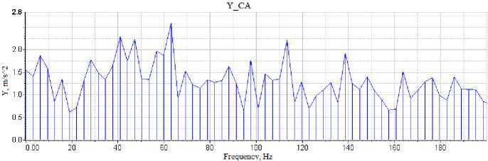
Рис. 7. График спектра амплитуды виброускорений случайного процесса пиковых значений датчика № 1 по направлению вертикальной оси Y за время движения ЭУ от t 0 = 7,8 с до t 1 = 10,5 с на участке разгона. Пуск ЭУ 20.09.2024 г.

Fig. 7. Graph of the amplitude spectrum of vibration accelerations of a random process of peak values of sensor #1 along the vertical Y-axis during the PP movement from t 0 = 7.8 s to t 1 = 10.5 s during the acceleration section. PP start-up date: September 20, 2024

The greatest amplitude of the resonant response of the test object simulator is А Y = 2.589 m/s² at a frequency of f = 63.0 Hz. However, a sufficiently large number of resonant peaks with frequencies from 6.3 to 200 Hz are simultaneously present, from which it is difficult to isolate a specific cause. To assess the influence of front shoe vibrations transmitted to the test object simulator, the dynamic coefficients of the transfer function were determined; they were calculated based on the power spectra of the corresponding signals from sensors № 2 and 1 [8; 10; 22; 23].

The frequency range chosen was significantly larger than necessary for calculating the transfer function, since the power spectrum of the corresponding vertical vibration acceleration signals of sensor № 2, located in the front shoe, is significant in the frequency range from zero to 100 Hz. Figure 8 shows the dynamic coefficients of the transfer function H(f) of vertical vibration accelerations, where the input signal is the power spectrum (PS) of sensor № 2, and the output signal is the power spectrum of sensor № 1.

Y1 CM/Y2 CM-H(f)

0.0503 j                             “

□ .□2-

0     100    200    300 Frequency, Hz

Рис. 8. График динамических коэффициентов передаточной функции Н ( f ), определенной по спектрам мощности виброускорений случайного процесса пиковых значений по направлению вертикальной оси Y от датчика № 2 к датчику № 1

Fig. 8. Graph of the dynamic coefficients of the transfer function H( f ), determined from the power spectra of vibration accelerations of a random process of peak values in the direction of the vertical Y axis from sensor No. 2 to sensor No. 1

The vertical axis shows the dimensionless transmission coefficients, and the abscissa axis shows the frequency in Hz. The graph shows that disturbances from the front shoe to the test object simulator are transmitted with significant attenuation. For subsequent analysis and identification of the dynamic state features of the test object simulator during acceleration of the experimental setup during a movement time of Δ t = 2.65 s based on the results of recording the vertical vibration acceleration signal of sensor № 1, we apply wavelet transforms with the Morlet basis function. An example of the application of wavelet transforms for a detailed analysis of vibration accelerations of the BC 327 sensor is given in [25–27].

Fig. 9 shows the graphs of the dependence of the amplitude and pulse signal of vibration acceleration of sensor № 1 in the direction of the Y axis of the test object simulator depending on the time (and, accordingly, the speed) of the experimental setup movement.

The volumetric picture presented in Fig. 9 is a set of instantaneous amplitude-frequency characteristics (AFC) of the wave field reflecting the dynamic response of the test object simulator at the installation point of sensor № 1. The time axis in seconds (with a resolution of up to 1 μs) corresponds to the position of the experimental setup at the track mark. Time marks correspond to the current speed of the carriage. The vertical axis reflects the amplitude of vibration accelerations with a dimension of m/s² (with an error of up to 5 % in the frequency range from 10 to 2000 Hz, with an error of up to 10 % in the frequency range from 2 to 10 Hz). On the left along the graph is the frequency axis in Hz. For each moment in time along the frequency axis, you can select a graph representing the instantaneous AFC of the vertical vibration accelerations of a given sensor with the cursor. The numerical values of all parameters are displayed on the horizontal panel located below the graph. The vibration acceleration amplitude is additionally color-coded according to the vertical bar. Another cursor, pointing along the time axis, reflects the change in vibration acceleration amplitude along the Y -axis of the harmonic with a fixed frequency as the experimental setup accelerates. The harmonic with the lower frequency f

= 1.0 Hz has the highest power density spectrum and the highest energy density spectrum of the vibrations; it reflects the dynamics of the increase in the vibration acceleration amplitude of the test object simulator depending on the experimental setup acceleration rate. Figure 10 shows a graph of the change in the amplitude of the vertical vibration acceleration signal of the test object simulator depending on the experimental setup acceleration rate.

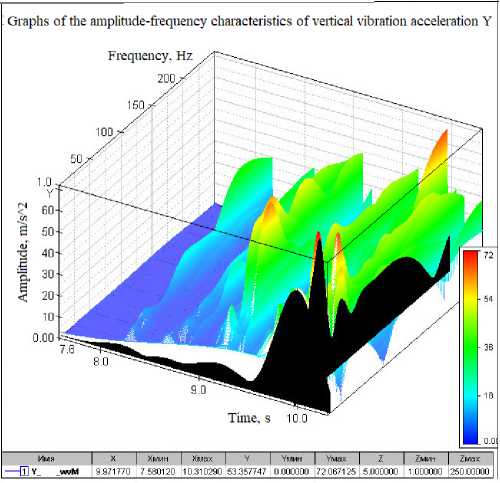
Рис. 9. Графики зависимостей амплитуды и частоты случайных виброускорений по направлению вертикальной оси Y по сигналам датчика № 1 за время движения ЭУ Δ t = 2,65 с на участке разгона. Пуск ЭУ 20.09.2024 г.

Fig. 9. Graphs of the dependences of the amplitude and frequency of random vibration accelerations in the direction of the vertical Y axis based on the signals from sensor No. 1 during the movement of the power plant Δt = 2.65 s in the acceleration section. Start-up of the power plant on September 20, 2024

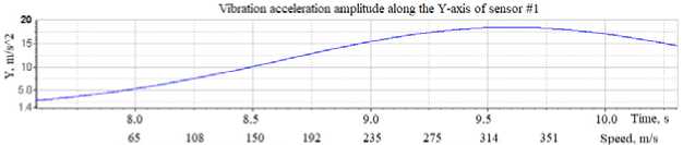
Рис. 10. График зависимости амплитуды случайных виброускорений по направлению вертикальной оси Y датчика № 1 за время движения ЭУ на участке разгона. Пуск ЭУ 20.09.2024 г.

• Fig. 10.    Graph of the dependence of the amplitude of random vibration accelerations in the direction of the vertical Y axis of sensor No. 1 during the movement of the power plant in the acceleration section. Power plant launch on September 20, 2024

The ordinate axis shows the vibration acceleration values in m/s2, and the abscissa axis shows the track carriage movement time in seconds. Below, another scale is placed, reflecting the relationship between time and the carriage speed. It should be noted that the speed values in relation to time are determined by calculation. The start of the experimental setup based on the vibration acceleration signal marks for different directions of sensor № 1 was performed at the time t0 = 7.8 s. Autonomous vibration acceleration sensors BC 327 are switched on immediately before the start, and the reading is selected for each sensor based on the presence of vibration acceleration signals. The error in matching the track carriage speed due to a shift in the start time selection can reach up to 10 %. In Fig. 9, for the time t = 9.972 s, corresponding to the experimental setup speed according to the calculation V = 388 m/s and the position of the carriage at the track mark L = 514 m, the following graphs are highlighted. The amplitude and frequency graph is a graph of the frequency response of the vertical vibration acceleration signal Y of sensor № 1, which corresponds to the shock wave response as the carriage crosses the sound barrier. The amplitude of the harmonic with a frequency of f = 1 Hz was AY = 17.2 m/s², while for f = 3.5 Hz it was AY = 31.4 m/s². Further, as the frequency increased, at f = 4.0 Hz it was AY = 43.05 m/s², and at f = 5.5 Hz it reached AY = 54.2 m/s². These frequencies are close to the natural frequencies of the front and rear shoes. The harmonic disturbance transmission coefficients from the front shoe (sensor № 2) to the test object simulator (sensor № 1) for the frequency range from 1 to 6.3 Hz, determined on the basis of Fourier transforms, are presented in Fig. 8. They are transmitted with attenuation k = 0.02. As the frequency increases, the contribution of the vibration acceleration components from the effects of aerodynamic forces and moments on the test object simulator increases. Thus, at the resonance response frequency f = 39.0 Hz, the amplitude increased to the values AY = 66.9 m/s², and at the resonance frequency with f = 41.5 Hz it was equal to the maximum value AY = 68.36 m/s². From this, it can be concluded that at the time t = 9.972 s, at the carriage speed equal to 340–350 m/s, the amplitude of the vibration accelerations of the response of sensor № 1 along the vertical channel is maximum. In the composition of the dynamic response signals of sensor № 1 from vertically directed impacts, the resonances from the contact interaction of the shoes with the rail guide at frequencies f = (4.0–5.5) Hz are significantly less than from aerodynamic impacts at frequencies f = (38–41.5) Hz (Fig. 10). Up to and including t = 9.972 s, the influence of very low-frequency impacts on the test object simulator is not detectable. Therefore, we conclude that the increase in the amplitude of vertically directed vibration accelerations for the frequency range starting at f = 39.0 Hz is due to a restructuring of the physical pattern of airflow around the test object simulator (Figure 11).

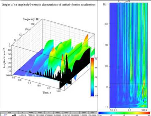
Рис. 11. График зависимости амплитуды виброускорений случайного процесса наибольших пиковых значений по направлению вертикальной оси Y по сигналам датчика № 1 за время движения ЭУ на участке разгона

• Fig. 11.    Graph of the dependence of the amplitude of vibration accelerations of a random process of the largest peak values in the direction of the vertical Y axis according to the signals of sensor No. 1 during the movement of the power plant in the acceleration section

Fig. 11 shows the frequency response graph of the vertical vibration acceleration signal from sensor № 1, corresponding to the moment of the experimental setup movement at t = 10.059 s. A flat representation of the volumetric graph is shown on the right. This allows one to identify the harmonic components of the vertical vibration acceleration response signal with the highest amplitudes (by color). The graph cursors are uniquely linked. This allows one to quickly examine the vibration pattern and relate the frequencies of the harmonic components to the amplitude and instantaneous velocity of the carriage.

In this case, the increase in the amplitude of vertical vibration accelerations of sensor № 1 is due to a restructuring of the physical pattern of air flow over the surface of the test object simulator. The restructuring of the shock waves from a normal shock to an oblique shock system does not occur simultaneously. Thus, at time t = 10.059 s, at a velocity of V = 380–388 m/s and a frequency of f = 58.0 Hz, the resonant response amplitude is А Y = 67.2 m/s².

Conclusion

Comparing the amplitude-frequency characteristics obtained on the basis of Fourier transforms (see Fig. 7) [8–10; 22–23] with the data determined using wavelet transforms shown in Figs. 9 and 11, we note that spectral analysis based on Fourier expansions of the convolution of the measured vibration acceleration signals and the impulse function significantly underestimates the values of the maximum amplitudes. Thus, the response of sensor № 1 in the vertical channel at a frequency of f = 41 Hz corresponds to an amplitude of AY = 2.6 m/s², obtained by the Fourier transform method using the statistics of the maximum vibration acceleration values for the signal recording considered in the article, while the maximum amplitudes calculated by wavelet analysis are higher and differ by more than an order of magnitude. It should also be noted that in this case, the vertical vibration acceleration amplitudes were measured by a sensor located on the axis of the cantilever beam, offset 2.5 times closer to the embedment relative to the center of mass of the test object simulator. Given that the simulator is a solid rod, we can assume its bending according to the first mode. In this case, the amplitude of the vertical vibration displacements of the test object simulator's center of mass must also be increased by 2.5 times. This will lead to an increase in the effective maximum stresses and, accordingly, a decrease in the safety margin.