Fusion-Based Sensor Selection for Optimal State Estimation and Minimum Cost (Intelligent Optimization Approach)

Published Online April 2012 in MECS

Today target localization by using sensor fusion systems is one of the main issues of tracking scenarios. Estimation accuracy, sensor characteristics and cost of sensory system are three important criteria help for optimal sensor selection in a sensor data fusion problem. Sensor selection system designers are weighting these three criteria and some other factors in every situation.

In a target tracking application, observations about angular direction, range, and range rate are used for estimating a target’s position, velocities, and accelerations in one or more axes. The Collected observations from various similar or dissimilar sensors can be used in a sensor data fusion system to make a better decision. Many applications and different methods of sensor data fusion are presented in [1-5].

In all of sensor fusion methods, sensors equipped in the mobile robot or a manufacturing system are used in sensor fusion. However, there are some considerations by using any type of sensors for sensor fusion. For instance, it is desirable to minimize the cost of the sensory system. Therefore, a sensor selection technique before fusing sensor measurements is very useful in order to approve such considerations. Various strategies and approaches have been proposed for the sensor selection problem in [6-9]. A sensor selection algorithm based on the Modified Riccati Equation (MRE) is used to allocate two sensors equipped on a moving platform to track targets in [6]. Another sensor selection technique incorporated with sensor fusion is introduced by Takamasa Koshizen in [7]. The Author has extended The Gaussian Mixture of Bayes with Regularized Expectation Maximization (GMB-REM) as a robot localization system in terms of the external sensor selection task to reach a minimum error in the position of the robot.

This paper is organized as follows. In the next section, we briefly describe the state vector fusion method based on the Extended Kalman Filter that was utilized in our work. We show how two sensor measurements can be fuse to have an accurate state estimation. Section III describes the sensor selection concept. In section IV, we precisely formulate our proposed method for the sensor selection problem. We consider a target localization scenario and describe the sensor selection problem as a multi-objective optimization problem. Section V presents the simulation results from the application of the proposed method to the case of two sensors, and then we provide our conclusions and the efficiency of the proposed method in section VI.

• II.    Sensor Data Fusion

The problem of target tracking using measurements from sensors is of considerable interest in many military such as tracking aircrafts, missiles and unmanned aerial vehicles. It is also useful in civil applications such as robotics, air traffic control, air surveillance, and ground vehicle tracking. A total idea of two sensor data fusion is depicted for target tracking in Fig. (1).

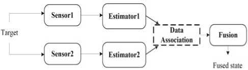
Figure 1． Concept of two sensor data fusion for target tracking [5]

There are generally two broad approaches for the fusion of data: measurement fusion and state-vector fusion. With the former approach, the measurements are basically combined without much processing, and the optimal state vector of target position is obtained. Statevector fusion is preferable in practical situations that the volume of data to be transmitted to the fusion center would be very large. In such a system, each sensor uses an estimator that obtains an estimate of the state vector and its associated covariance matrices (of the tracked target) from the data of that associated sensor. Then these state vectors are transmitted over a data link to the fusion center [5].

Suppose that for a given target tracking scenario, we have an autonomous robot that two sensors such as sonar with different accuracy are installed on it. Using each of these sensors, we would have two estimations from the target states with known and different accuracy. The state vector fusion problem in this scenario will be a weighted sum of the two independent state estimates. Fused state and covariance matrix are computed using the following expressions:

A p A -J Al/A1     A О \-1 / A 0     A 1 \

X f = X ¹ + P ¹ ( p ¹ + P ² ) ( X ² - X ¹ )

ˆ

P f = P 1 - p l ( P 1 + P 2 )-

1 P ¹

Where, X ^{ˆ 1} and X ^{ˆ 2} are the estimated state vectors of estimator 1 and sensor 2 with measurements from sensor 1 and sensor 2, respectively, and P ^ˆ1 and P ^ˆ2 are the corresponding estimated state error covariance.

• III.    Sensor Selection

In sensor management and sensor data fusion concepts, sensor selection is usually based on the accuracy and performance of each sensor. Although this accuracy is based on certain environmental and sensor related parameters, it does not necessarily mean that the sensor with the highest accuracy also yields the best performance in a sensor data fusion system. With an incorrect sensor selection scheme, it is probable that the fused estimate error be more than the achieved estimation error by each of the sensors.

Another issue here is a cost-benefit tradeoff. In practical situations, usually designers try to obtain the best performance against minimum cost of a sensory system. Also in tracking scenarios, the sensor selection process would be performed based on sensory characteristics. For example, for a given target tracking scenario, one is able to identify the best sensor with a high accuracy in range measuring, in the meantime the other sensor might be used for exact bearing measurements.

• IV.    Problem Statement

The proposed algorithm for sensor selection is based on state vector fusion. For a given stationary target, an optimal state estimation is achievable if we minimize the fused covariance P ^{ˆ f} . It is obvious from the (2) that the fused state estimate X ^{ˆ f} is directly relative to the fused covariance. Therefore, minimum fused covariance yields an accurate state estimation.

We state the following assumptions:

• 1)    We have a robot equipped with a sensor that has a known performance, named sensor 1 .

• 2)    A stationary target is placed in an unknown location that is able to be found with sensor 1.

• 3)    The initial position of the robot is available.

• A.    Target Position Initialization

Position estimate of the target and its covariance must be properly accomplished for sensor selection. The full set of two dimensional kinematic model of a robot is given by:

/ = tozb + wz(3)

vxi =(fxb + wx )cos/-(fyb + wy )sin/ vyi =(fxb + wx )sin / -(fyb + wy )cos/

X i = Vxi(6)

yi= vyi(7)

®zb is the measured angular rate and fxb and fyb are the measured specific force in body axes of the robot. wx , wy and wz are dynamic noise of internal sensor measurements. vxi and vyi are the robot velocity and xi and yi are the position of the robot in a space-fixed reference frame [10].

The robot is equipped with a range/bearing sensor. Laser range finders and sonar sensors are two examples of range/bearing sensors that might use on the robot. Given the robot position X _R = ( x_R , y_R ) and its orientation / , the observation of range, z r and bearing, z ₆ can be modeled as:

Z =

z _r

. z9

^^{( X} R - ^X t ^{) 2 + ( y} R - yt ^{) 2} arctan(—— y t )- ) - /

^{( X} R ^- x t )

w _r

. w9

where w r and w ₉ are uncertainty in sensor measurements. According to (3)-(7) and (8), the state vector of our system is X _R = [ x _R y _R v _X R v _X R / ] and observation vector is Z = [ z r z _e ] .

Given the (8), a target estimation model g _t , maps the robot position and relative observation to target position estimate. Therefore, the estimate of the target position is:

X t = g t (Xr,z)                                 (9)

and its covariance is :

P _t = A .P 0 . A T + B .R. B T                       (10)

Where P₀ is initial covariance of robot states, A and B are Jacobian of g _t evaluated around state vector and observations respectively.

B. Nonlinear Equation System Derivation

Covariance of observation noise or dynamic noise of measurement for sensor 1 and sensor 2 is defined by R1 and R2, respectively :

R i =

^O r 1 0

0          0 *2 0

, R 2 = ' ²

^O 9 1 J        L ^{0   CT} e - 2

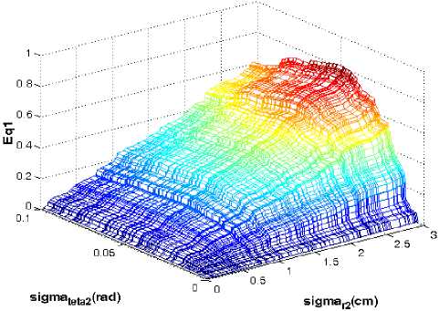
Figure 2 ． Surface plot of Eq1

where ( o r , o_e ) are standard deviation of range and bearing measurements respectively. According to (8) and (11), we will have two different observation models for sensor 1 and sensor 2 :

Z s2 ( k ) =

Z si ( k ) =

z r ( k ) "	J-	M r$ 2 ( k )
z g ( k ) j	+	L W 9 s 2 ( k ) _
z r ( k )	+	■ W rS 1 ( k ) "
z g ( k ) _		_ w 9 s 1 ( k ) _

,

Therefore, covariance estimates for target position by sensor 1 and sensor 2, P _{t 1} and P _{t 2} , will not have the same values. As we said before, sensor 1 has a known accuracy and is available, hence R1, P _{t 1} and Z _S1 are

non-parametric and take true values. But R2, P _{t 2} and

Z _S2 are parametric values. Further details in the

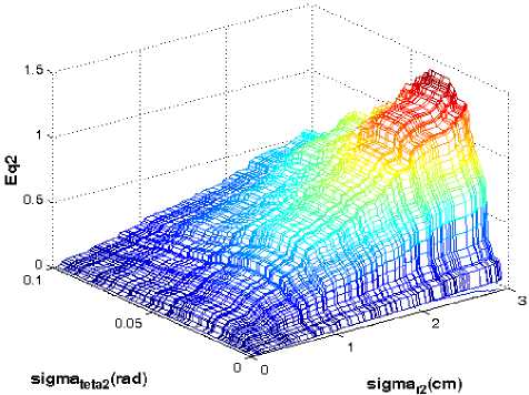
Figure 3 ． Surface plot of Eq2

calculation of P _{t 2} are given in Appendix. Also according

to (2), P^{ˆ f} will be a 2×2 parametric matrix based on ^{( o} r 2 , ° g 2 ).

^{P f} = ^{f ( o} r 2 , ^o 9 2 )

The main diagonal of P^{ˆ f} is consist of two nonlinear functions. After some simplifications and for a given value of random function, P^{ˆ f} takes on the different forms.

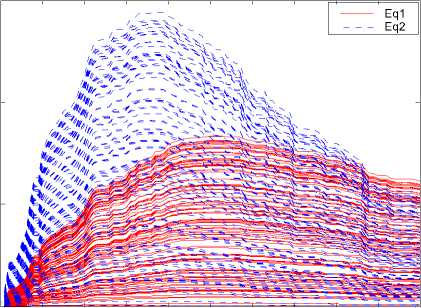
Indeed, Fig (2) and Fig. (3) shows variations of original diagonal elements of the fused covariance matrix into ( o _r 2 , o_g 2 ). If we plot these two surfaces in a common frame, some crossing points will appear. It proves that the equation set (16) has more than two answers. Fig. (4) shows these cross points.

Now, we try to minimize the fused covariance defined by (13) to have an optimal estimation of target position. Therefore, we can consider the sensor selection problem as a nonlinear multi-objective optimization problem. In

1.5

other words, ( o r 2 , o_g 2 ) must be specified in a manner

that the partial derivation of (13) goes

to zero:

Eqi

Eq 2

d 2 P f ( 1,1 ) ) = 0

5 ° r 2 ^do g 2

d2 (p f (2,2)) = 0

^{d o} r 2 ^{d o} 9 2

For the above equation set, because of high nonlinearity, it is difficult to calculate o r 2 and o_g 2

0.5

0     10 20 30 40 50 60 70 80 90 100

Number of Pairs of (sigmar2,sigmateta2) Values

Figure 4 ． Cross points of surface Eq1 and surface Eq2 in a common frame

analytically and the response of equation set is highly correlated to initial values. Fig. (2) and Fig. (3) show the values of specified Eq1 and Eq2 for a given and limit band o^{f (} O _r 2 , O g 2 ).

According to the above proofs, we propose multiobjective optimization approaches for solving nonlinear equation sets (14).

• B.    Transformation into a Multi-Objective Optimization Problem

The purpose of multi-objective optimization problem is to seek design vector X * = [ X * , X 2 , • , X n ] T according to k object functions f_i that must be minimized within a given set of m equality and p inequality constraints that restrict the problem. A mathematical formulation of the multi-objective optimization is :

find           X *

optimize    F ( X )                             (15)

Г g i ( X ) < 0 ( i = 1,2, • , m )

subject to     [ i j X ) = 0 ( j = 1,2,..., p )

where X * e^ ⁿ is a design variable vector, F ( X ) = [ f 1 ( X ) f 2 ( X )>••• , fk ( X )] T is object function vector and g i ( X ) and h ( X ) are equality and inequality constraint, respectively. With no loss of generality, we can assume that all of the object functions should be minimized. Such multi-objective minimization problems are classified as Pareto solution problems and for achieving the optimal solution, some definitions such as Pareto front, Pareto set, Pareto optimality and Pareto dominance are used.

In multi-objective problems, heuristic optimization methods, particularly genetic algorithms (GAs) be used extensively during the last decades to search for optimum solutions [11] – [15].

Genetic algorithms which imitate the process of natural evolution have shown successful results in many optimization problems which are difficult to solve by the conventional methods of the mathematical programming. In this work we used Non-dominated Sorting Genetic Algorithm (NSGA-II) for solving systems of nonlinear equations (14) as a multi-objective optimization problem.

The complete NSGA-II procedure is given below:

BEGIN

While generation count is not reached

Begin Loop

• •    Create the offspring population Q_t (of size N) using the parent population P t (of size N),

• •    Combine parent P_t and offspring population Q_t to obtain population R_t of size 2N.

• •    Perform Non-dominated Sorting on R_t and assign ranks to each Pareto front with fitness F i .

• •    Starting from the Pareto front with fitness F 1 , add each Pareto-front F i to the new parent population P t +1 until a complete front F i cannot be included.

• •    From the current Pareto-front F i , add individual members to new parent population P_t+1 until it reaches the size N.

• •    Apply selection, crossover and mutation to new parent population P_t+1 and obtain the new offspring population Q_t+1.

• •    Increment generation count.

End Loop

END.

• V.    Simulation And Results

In this section we define the sensor selection problem as a multi-objective optimization problem and we present simulation results to validate the theory developed in the previous sections.

We formulate the multi-objective optimization problem as follows :

Г Optimize ^{f (} x ) = ^{( f} i⁽ x ), ^f 2⁽ x ) )

[ subject to x = ( p r ₂, ct_{q 2} [ Minimize abs( f 1 ( x ))

) eQ

[ Minimize abs( f ₂( x ))

f ₁ ( x ) and f ₂ ( x ) in this formulation take the values Eq1 and Eq2 in (14) respectively.

The upper and lower bounds are considered as follows :

Lower Band : ^{[ p} r 1 ^p 0 1 ^{]                          (17)}

Upper Band : [ n x p r 1 m x ct_{6 1} ]                    (18)

where n and m are positive real values.

Again, consider presenting equations in Appendix that are utilized for relative range and bearing ( z_{r 2} , z_{t 2} ) calculation between robot and target using sensor 2. As we can see, a random function with zero mean and specified variance ( p r 1 , p_{6 1} ) has been used in these equations. Therefore the performance of proposed method must be evaluated by Monte Carlo simulation. For different random function values, several object functions will be derived and multi-objective optimization algorithm will be served to solve the derived nonlinear equation set.

For simulation, consider the scenario presented in Fig. (5). In this scenario, a target is placed in position (100,200) and we want to estimate the location of the target by a robot that is placed in position (0,0).

Target Localization Scenarion

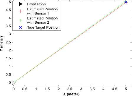
Figure 5 ． Multi-sensor target localization scenario

Monte Carlo simulation iterated 100 times. The simulation parameters and characteristics of first sensor are shown in table I. The values of the parameters used in the simulation by genetic algorithm are given in table II.

All solutions in a Pareto set are equally optimal. It is up to the designer to select a solution in the Pareto set depending on the application. In this work we choose the mean of solutions as a final answer and select the second sensor based on this answer.

TABLE I.     Simulation Parameters and characteristics of sensor 1

Sampling Period	Δ t ( k )	0.01 Sec
Noise STD dev in the range measurement of sensor1	σ r 1	2 cm
Noise STD dev in bearing measurement of sensor1	σ θ 1	0.02 rad
Initial position STD dev of Robot	σ x , σ y	1 cm, 1 cm
Initial velocity STD dev of Robot	σ Vx , σ Vy	1e-3 m/s , 1e-3 m/s
Initial heading STD dev of Robot	σ ψ	1e-4 rad , 1e-4 rad
Upper and Lower bounds in optimization algorithm	U b , L b	5 cm , 0.1 rad

TABLE II.     V alues of the P arameters U sed in the

Objective 1

x 10-3

S imulation by G enetic A lgorithm

Parameter	Value
Population Size	30
Number of Generations	300
Number of Variables	2
Function Tolerance	1e-4

Some of the solutions obtained by a single run and for a given object function as well as the function values (which represent the values of the system’s equations obtained by replacing the parameter values) are presented in Table III. The algorithm provides optimal Pareto curve as shown in Fig. (6).

A SINGLE RUN FOR A GIVEN OBJECT FUNCTION

Figure 6 ． Optimal Pareto solutions for the multi-objective optimization problem

For more analysis, average Pareto distance and spread of generated individuals in genetic algorithm are shown in Fig. (7).

Average Distance Between Individuals

0.4

I Q

I

0.3

0.2

0.1

**уе>А(*^«й^ав^^^

50         100        150

*e«»*6^***f

200       250       300

'о CZ)	Variables Values		Function Values		Fusion Covariance		Target Position Estimation Covariance By Sensor 2
	σθ 2	σ r 2	Eq1	Eq2	P ˆ f ( 1,1 ) P ˆ f ( 2,2 )		P ˆ 2 ( 1 , 1 ) P ˆ 2 ( 2 , 2 )
	2.930	0.028	3e-06	0.0098	2.6359	2.5393	5.1988	5.4541
	3.021	0.020	0.007	1e-06	2.612	2.5168	5.5303	5.7221
	2.934	0.021	3e-04	0.007	2.6349	2.5387	5.2274	5.4173
Sol	2.943	0.021	0.001	0.0063	2.6325	2.5363	5.2571	5.4514
1	3.000	0.020	0.005	0.0015	2.6174	2.5219	5.4561	5.6494
	2.930	0.028	3e-06	0.0098	2.6359	2.5393	5.1988	5.4541
	2.960	0.022	0.002	0.0050	2.628	2.532	5.3133	5.5172
	2.991	0.020	0.005	0.0022	2.6198	2.5242	5.4245	5.616
	3.691	0.021	4e-07	0.028	2.345	2.470	8.626	7.484
	3.090	0.055	0.068	3e-07	2.458	2.599	6.584	4.610
	3.090	0.055	0.068	5e-10	2.458	2.599	6.584	4.610
Sol	3.122	0.021	0.025	0.003	2.454	2.587	6.246	5.429
2	3.094	0.025	0.031	0.001	2.460	2.594	6.187	5.251
	3.319	0.021	0.013	0.015	2.412	2.542	7.027	6.103
	3.416	0.022	0.009	0.020	2.393	2.522	7.437	6.430
	3.082	0.031	0.040	3e-07	2.462	2.598	6.220	5.083
	2.903	0.057	34-10	0.025	2.578	2.606	5.000	5.657
	3.017	0.034	0.015	1e-09	2.548	2.577	5.447	5.869
	2.902	0.025	4e-08	0.011	2.578	2.607	5.088	5.378
Sol	3.014	0.021	0.009	1e-04	2.549	2.578	5.484	5.743
3	3.017	0.026	0.012	2e-05	2.548	2.577	5.474	5.800
	3.017	0.034	0.015	1e-09	2.548	2.577	5.447	5.869
	2.919	0.026	0.001	0.009	2.573	2.603	5.144	5.444
	2.950	0.022	0.004	0.005	2.565	2.595	5.256	5.525

Average Spread: 0.048299 0.8

0.6 p

0.4

0.2

50        100       150       200       250

Generation

Figure 7. Average Pareto distance and spread of generated individuals

Table IV shows the characteristics of selected sensor. The results are obtained after 100 Monte Carlo simulation runs.

TABLE IV.    V alues of the P arameters U sed in the

S imulation by G enetic A lgorithm

Noise STD dev in the range measurement of sensor 2	σ r 2	3.3939 cm
Noise STD dev in bearing measurement of sensor 2	σ θ 2	0.0396 rad

Fig. (8) depicts the time histories of target position estimation errors with ± 3 σ bounds for state vector fusion algorithm scheme when we fuse the obtained measurements by sensor 1 and sensor 2. Sensor 2 is selected by the proposed sensor selection algorithm.

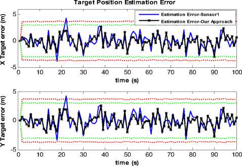
Figure 8 ． Target position estimation error – sensor 1 and our approach

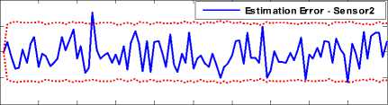
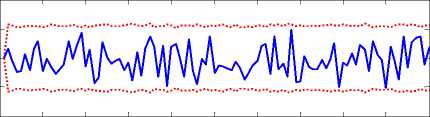
From the results presented in Fig. (8), one can see that satisfactory accuracy of position estimation has been obtained using the proposed sensor selection algorithm. Fig. (9) presents estimation errors with ± 3 σ bounds when we only use sensor 2 for target position estimation.

Target Position Error - Sensor2

g

Я

E5

x

-5

-10

0     10 20 30 40 50 60 70 80 90 100

time (s)

0     10 20 30 40 50 60 70 80 90 100

time (s)

Figure 9 ． Target position estimation error – sensor 2

g

-10

Using 100 Monte Carlo simulations, Estimation accuracy was measured by the total RMSE in the position estimates of the target. Results are presented in table V.

POSITION ESTIMATION

	Estimation with Sensor 1 measurements	Estimation with Sensor 2 measurements	Estimation with fused measurements
X Position RMSE	1.4050	2.2224	1.1037
Y Position RMSE	1.4114	2.1333	1.0930

• VI.    Discussions and Conclusion

A new heuristic algorithm for sensor selection problem has been proposed in this paper and its success investigated by some simulations. Given a specified sensor, we selected another one to pair with it. Considering a design area for sensor selection, we defined a multi-objective optimization problem and selected a perfect pair of sensors for optimal state estimation. Using the state vector fusion method, accurate target position estimation performed by the selected sensors such that a trade-off between cost of the sensory system and estimation error is created.

Proposed method gives us more solutions for the sensor selection problem that all of them are optimal, but in this work we choose the mean of solutions to make a sensory system.

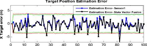
It is worth to mention the necessity of using our approach for selection of a perfect pair of sensors in position estimation problems. In section V, we considered a design area for sensor selection. In this section, we ignore our sensor selection algorithm and put the ( σ r 2 , σ_θ 2 ) equal to upper bound values of design area. Estimation error results with ± 3 σ bounds and total RMSE for this condition are presented in Fig. (10) and table VI respectively.

Target Position Estimation Error

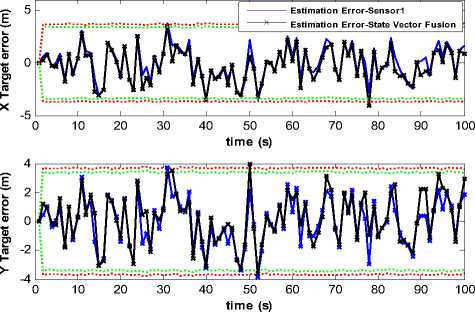
Figure 10 ． Target position estimation error : ( σ r 1 = 2 cm , σ_θ 1 = 0.02 rad ) and ( σ r 2 = 5 cm , σ _θ 2 = 0.1 rad )

table vi. RMSE values for target position ESTIMATION : ( σ _{r 1} = 2 cm , σ_{θ 1} = 0.02 rad ) AND ( σ _{r 2} = 5 cm , σ _{θ 2} = 0.1 rad )

	Estimation with Sensor 1 measurements	Estimation with Sensor 2 measurements	Estimation with fused measurements
X Position RMSE	1.5801	7.2762	1.9143
Y Position RMSE	1.5948	5.8132	1.9626

It is obvious from Fig. (10) and table VI that the state vector fusion algorithm has not successful results for any arbitrary pairs of sensors. While our proposed algorithm always select a perfect pair of sensors such that gives optimal fusion results.

Propriety between the range and bearing measurement accuracy of selected sensor is another important ability of our proposed algorithm. In the state vector fusion algorithm, incorrect selection of sensor 2 may cause to undesired estimation results, while the cost of sensory system is reduced.

For example, consider the presented characteristics of sensor 1 in table I. Here we use a low cost sensor 2

described by a r 2 = 10 and a₆ 2 = 0.001 in which the propriety between range and bearing measurements is not regarded. In this case, Fig. (11) shows attained estimation accuracy by state vector fusion algorithm.

time (s)

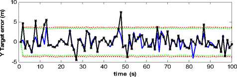
Figure 9 ． Target position estimation error :

( a r 1 = 2 cm , a_{6 1} = 0.02 rad ) and⁽ a r ₂ = 10 cm , a _{6 2} = 0.001 rad )

As we can see from this figure, fused estimation error is higher, as compare with the case that sensor 1 is used for position estimation, where errors exceed the ± 3 a confidence bounds.

Our approach is applicable for any type of sensors and selection has done based on the accuracy of sensors in range and bearing measurements. As we know, increasing in measurement accuracy of sensors makes them expensive. Our approach is very valuable for a decision maker to select proper sensor suites according to requirements. Therefore, by utilizing the proposed algorithm, we can select a pair of sensors with minimum cost to have an optimal estimation in target tracking problems.