Ground vibration test results for modal updating of aircraft

Designing aircraft (AC) involves meeting requirements for dynamic loading of structures and controllability of spacecraft (SC), as well as the strength and aeroelastic stability of aviation equipment (AE). To solve these problems, computational dynamic models of AC are used, built according to the technical documentation of the products. Since such computational models may, for known reasons, not adequately reflect the dynamic properties of the designed aircraft, they are later adjusted based on test results. Modal tests, which are an integral part of ground experimental development of AC, are used to correct the computational models of spacecraft.[1]. Experimental modal analysis results are also used to adjust the computational models of aircraft, and these adjustments are carried out throughout the entire product lifecycle: design (dynamically similar models), prototype production, serial production and design modifications [2; 3]. A review of ground modal testing methods is presented in the monograph [4]. During the trial operation phase, the computational models can also be adjusted based on the results of operational modal analysis in flight tests [5].

To fix the inaccuracies in modelling, various methods for correcting computational models have been developed [6–9]. The well-known correction methods can be divided into two categories: stochastic and deterministic. Stochastic methods are based on the idea that experimental data is random and contains inevitable errors [10–11]. Deterministic methods involve an iterative process of minimising a target function, which is the sum of the squares of differences between experimental data and modelled data [12–14]. The convenience of this approach lies in the fact that heterogeneous parameters, such as natural frequencies and structural responses to dynamic loads, can be included in the target function at the same time [15].

Experimental modal analysis method

The task is to experimentally determine the initial data to correct the aircraft's calculation model using a deterministic method, based on the equations of natural oscillations.

AY + CY = 0                                 (1)

and the general problem of eigenvalues

(С - pA) W = 0.

Here Y(N) is the vector of the structure's point displacements; A(N×N) and C(N×N) are the inertia and stiffness matrices; N is the number of degrees of freedom of the model; p are the eigenvalues (natural vibration frequencies); W is the matrix of eigenvectors. Corrections can be applied to the inertia and stiffness matrices. As initial data for correcting such a model, dynamic characteristics like generalized masses, natural frequencies and vibration modes obtained from modal testing can be used. However, these characteristics cannot all be used together in the correction because vibration modes are determined by the system's inertial and elastic properties, so they can only serve as checks.

The identification of natural vibration frequencies is done using a multi-point harmonic excitation method. In this case, for describing the forced vibrations of the aircraft during testing, a differential equation is usually used.

AY + HY + CY = E sin ( ® t ) + F cos ( ® t ) ,                         (2)

the established decision of which is

Y = U sin ( ro t ) - V cos ( ro t ) .

Here, H(N×N) denotes the damping matrix, E(N) and F(N) are the vectors of in-phase and quadrature components of the excitation forces, ω is the frequency of forced vibrations; U(N) and V(N) are the vectors of in-phase and quadrature (real and imaginary in the complex representation of vibrations) components of the displacements of the structure points.

It should be noted that unlike equation (1), equation (2) includes a description of the dissipative properties of the dynamic system. Therefore, when defining the inertia and stiffness parameters based on test results, damping characteristics are taken into account, which are not provided for in the original equations (1). On this basis, we will consider the forced vibration equations of the AC during testing in the form

R = HY / ю,(4)

where R(N) is the damping force vector, which includes all forces that change in phase with the oscillation speed, and the properties of the damping matrix are determined from test results.

It is assumed that by selecting the excitation, a mode of forced single-phase oscillations is achieved

U = X V,(5)

where λ is a real number. In this case, differential equations (3), taking into account (4) and (5), correspond to a system of algebraic equations

(1+ X2)(C-ю2 A) V = XE - F,(6)

(1+ X2) HV = E + X F.(7)

Equations (6) and (7) allow for independently determining the elastic-mass characteristics of the aircraft and the damping characteristics. Article [16] explains the properties of forced monophase oscillations, ways to select the excitation and the procedure for experimental modal analysis, as well as the method for identifying the properties of the damping matrix.

The general characteristics of L natural vibration modes ( L ≤ N , usually L << N ) are determined in modal tests under conditions:

• 1)    if single-phase excitation ( F = 0) results in a phase resonance mode (λ = 0), then from (6) it follows that single-phase vibrations are natural vibrations ω = pi, V = Wi, i = 1, 2, …, L ;

• 2)    if near phase resonances (ω ≠ p i ) single-phase excitation leads to single-phase vibrations coinciding with natural vibrations, then, as follows from (6), the generalised mode masses are determined by the formula

X V ^T E

( 1 + 1 2 )( p 2 -ю ² ) V"

At the same time, damping is described by a generalized coefficient (7)

h i =

viT E

( 1 +^ ² ) V *²

Here V_i ^* is the quadrature component of displacements at the point where the tone of the oscillations is normalised.

If we assume that damping is small and the natural and free oscillation frequencies are equal, we can get a formula to estimate the generalized decrement of oscillations.

§ i =

2 n

4 P X

V ( P 2 -ю ²)²

;

- 1

• 3)    If near the phase resonances in single-phase excitation the single-phase oscillations don't match the natural oscillations, you need to introduce a quadrature component of the excitation to determine the generalised masses.

  ^a i ⁼

  
  

  V_i ^Τ ( λ E - F )

  
  

  (1 +λ ²)( p i ² -ω ²) V i ^*2

  
  
  
  

damping is no longer described by a generalised coefficient.

Regarding the test conditions considered, the following points should be noted:

• –    мeeting condition 1 is mandatory for determining the frequencies and modes of natural vibrations using the phase resonance method;

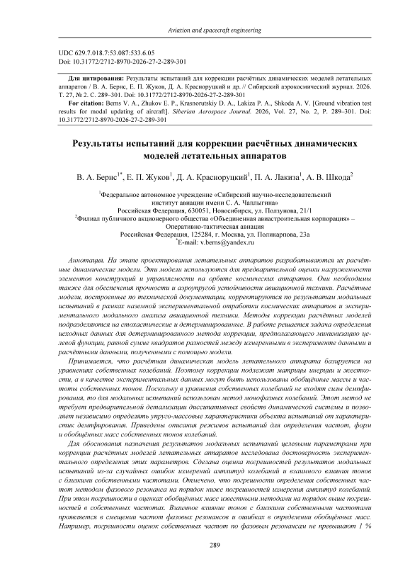
• –    based on the experience of AC modal tests, condition 2 is practically always met, i.e., in the vicinity of phase resonances, there is a range of frequencies where forced single-phase vibrations under single-phase excitation coincide with the natural vibrations (Fig. 1, ῶ – the ratio of vibration frequency to phase resonance frequency). This means that the generalised dynamic characteristics are determined by formulas (8–10).

  

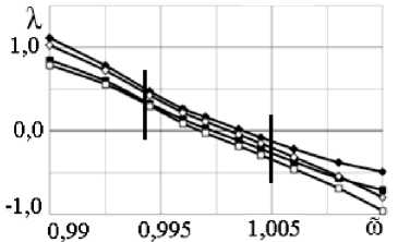
  Рис. 1. Монофазные колебания в окрестности фазового резонанса

  
  

Fig. 1. Monophase oscillations in the vicinity of the phase resonance

Results of modal tests for the correction of computational models

To justify using the results of modal tests – generalised masses and natural vibration frequencies – as target parameters for adjusting aircraft calculation models, it is necessary to establish the reliability of experimentally determining these parameters. Studies [17; 18] note that errors in test results are usually due to random measurement errors in forced vibrations and in selecting the excitation, as well as the mutual influence of tones with similar natural frequencies.

Studies on the errors of modal test results due to random measurement errors have shown that the errors in determining natural frequencies using the phase resonance method are an order of magnitude lower than the errors in measuring vibration amplitudes. At the same time, errors in the estimation of generalized masses using known methods (the monophase vibration method, the method of introducing a quadrature component of excitation, the fictitious phase resonance method, the complex power method) can exceed the errors in measuring vibration amplitudes by more than 1.5 times. Article [17] presents a methodology for determining generalized masses from the amplitude-frequency characteristics of aircraft, which allows the error in mass determination to be reduced, yet it remains significantly higher than the errors in natural frequencies.

The mutual influence of tones with similar natural frequencies mainly shows up in the shift of phase resonance frequencies, which are used to estimate these natural frequencies. It's worth noting that we mean not only the vibration tones of AC structures: modal tests for testing structures use elastic suspension systems, and for space structures, zero-gravity systems. This means that if in operational conditions the test objects have vibration tones like those of a rigid body with zero frequencies, under test conditions vibration tones appear as those of a rigid body on an elastic suspension. And the vibration frequencies are no longer zero. Therefore, when designing such suspension and zero-gravity systems, it is necessary to take into account that the influence of aircraft vibrations as a rigid body on their dynamic characteristics should not exceed the specified limit.

Let us assume that in the vicinity of the tone with number i, the AC vibrations are influenced by some tone with number j so that g = gi + wjgj, where g is the displacement of the test object's control point; gi and gj, are the generalized coordinates of the i-th and j-th modes; wij is a coefficient characterising the contribution of the j-th mode to the system's vibrations. Let's define the natural frequency and the generalized mass of the i-th mode, assuming the influence of the j-th mode can be neglected. We assume that the damping of each mode can be described by a generalized vibration decrement.

Let's introduce the notations:

_w 2 _a к =— , a j

p,         h     §,

& = —, n =—=—, n P i          P i a i    ⁿ

j

h j      ^ j   - ®

—T~ = —, ® = —. pjaj   ⁿ Pt

We will obtain an expression for the parameter of forced monophase oscillations under monophase excitation from the solution of the problem of forced oscillations of a system with two degrees of freedom:

Х(й) =

? 1R T j (( » )’

where

( < % ² - 1 ) ^[ (® ² - s ² ) ² + n^j s⁴ ] + к (( % ² - s ²) ^[ ( ( % ² -1 ) ² + n^j ]

^Tl( ® ) =-------------------------- —_j--------------_j-------- ,

^{[ k(}< % ^{j -} 1) ^{+ ( шj - s} ) ] ⁺ ( ^k n i +n j ^s2 )

7-2    2x2 .      2^7-2                       .     2\

T j (() =

n i ( ш - s ) + n j & k( ( - 1) +nn j & ( n i к + n j & )

^[ k( ( ^j - 1) + ( ( ^j - s ² ) ] ^j + ( k n i + n j s ² ) ^j

By letting λ pass through zero from positive to negative values, we find the relative eigenfrequen-ciesof the system, for which we solve the equation f (() = ((j -1)[(Йj-sj)j +n>4] + ^ ((j-sj)[(Йj -1) j+ nij] = 0.          (12)

Based on the analysis of the roots of equation (12), the following conclusions are made about the estimation of the natural frequency of the i-th tone p i ^*, determined by the zero crossing of the parameter λ, assuming that the j -th tone has little effect on the system's oscillations: if p i >  p j , then p j <  p i ^*<  p_i ; if p_i <  p j , then p j >  p_i ^* >  p_i ; if p_i = p j , then p_i ^* = p_i . If equation (12) has only one real positive root, which occurs when the parameters ξ, æ, η _i and η j satisfy the inequality

4d3 + j7c2 > 0, where j Lj L j кз          K K   s2(2 + ^) +1 + j^

d = зb1 + bj, c = jy b1   зb1 bj + b3’ b1 =       1 + ^

s4nj+ 2s2(1 + ^) + ^(1 + nj)        s4nj + sj^nj ’ b2 =----------------------------------, Ьз =-, j                 1 + ^                  31 then the natural frequency, determined by the λ crossing zero(pi*), can be the frequency of either the i-th or j-th tone. The frequency pi* corresponds to the i-th tone if both roots of the equation occur when æ < 1.

f 'R = 0

less, and for æ > 1 the equation (13) has a larger root. Otherwise, the i -th tone won't be detected during testing.

Figures 2 and 3 show the results of calculating the relative frequency p͂ i = p i^* /p i for different values of the parameters ξ, æ, δ i и δ j , which indicates that the natural frequency of the i -th tone is determined quite accurately. For example, for δ i ≤ 0.2 and ξ ≤ 0.5, the error in determining p i does not exceed 0.5% regardless of the ratio of the natural frequencies of the i -th and j -th tones.

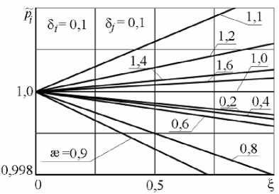
Рис. 2. Оценки собственной частоты при различных значениях ξ и æ

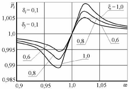
Рис. 3. Оценки собственной частоты в зависимости от параметра æ

• Fig. 2.    Estimates of the natural frequency at different values of ξ and æ

• Fig. 3.    Estimates of the natural frequency as the function of the parameter æ

To determine the generalised mass of the i -th mode under single-phase excitation, we use formula (8). Instead of the frequency ῶ, we introduce another frequency parameter Ω = ω/ p_i ^*, which is related to ῶ by the relation Ω = ῶ/ p͂ _i . This is because modal testing results determine not the exact value of the natural frequency of the i -th mode, but the value p_i ^*. For practical purposes, it is interesting to assess the accuracy of determining the generalised characteristics of the mode near the found natural frequency. For calculating the relative generalised mass, the formula obtained is ( a͂_i – the ratio of the determined generalised mass to the exact value):

_ т ( Q ) ^^^^^^ш ^^^^^^^^^^^^^^^^^^^^^^^^^^^^^^^^^^^^^^^^^^^^^^^^^^^^^^^^^^^^^в

а2(1 -Q)’

From the results of the calculation of the relative generalized mass shown in Figures 4 and 5, it can be seen that as ξ increases, the frequency range of forced vibrations, for which the generalized mass is determined with a pre-set accuracy, decreases. In addition, as ξ increases, this range shifts from the frequency p i^* to the sub-resonance area when p i >p j and to the post-resonance area when p i < p j . When the natural frequencies of the i -th and j -th tones get close, the accuracy of determining the generalized mass and the generalized damping coefficient near the tone's natural frequency decreases. The greatest deviation of the generalized characteristics from exact values for Ω ≈ 1 is observed at æ=1 and in the case of equal decay rates of the tones, which is determined by the expression

^^

ai =

1 +^ ^,

that is, the estimated generalised mass is always less than its exact value.

Comparing figures 2 and 3 with figures 4 and 5, we conclude that the influence of the j -th mode affects the accuracy of the generalised mass more than the accuracy of the natural frequency of the i -th mode. To obtain a_i with a 5 % error regardless of the relationship of natural frequencies, the value of ξ must not exceed 0.05.

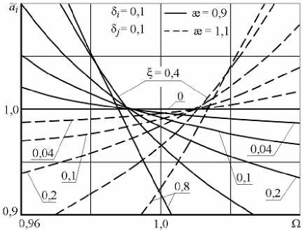
Рис. 4. Оценки обобщённой массы при различных значениях параметров ξ и æ

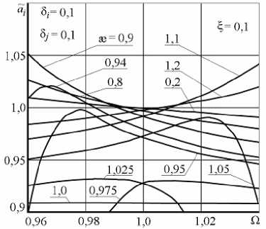
Рис. 5. Оценки обобщённой массы при различных значениях параметра æ

Fig. 4. Estimates of the generalized mass at different parameter values of ξ and æ

Fig. 5. Estimates of the generalized mass at different values of the parameter æ

The results of the research on errors in determining generalized characteristics suggest that the numerical values of the parameters ξ, æ, δ _i and δ j are known. The values of p_i and p j can be estimated from the frequencies of phase resonances, δ _i and δ j are calculated using formula (10), and the parameter ξ is determined from the measured value of λ. For example, when exciting oscillations at a frequency different from the resonance frequency, we arrive at the following expression to estimate the parameter ξ:

. = a (i -tf ² -Xn , ) P ( Xn j ж² - ж ² +tf² ),

a = (ж² (I )² +n>⁴ ; в = ( 1-tf² )² + n 2 .

So, using a system with two degrees of freedom as an example, the general characteristics of the natural vibration mode were determined, assuming that the effect of the other mode could be ignored. Therefore, a single-point excitation was used, and the natural frequency and generalised mass were calculated from the response at the force application point. The resulting calculation errors were explained by the mismatch between the number of degrees of freedom in the model and the original system (a single-degree-of-freedom model for a two-degree-of-freedom system).

Using the same example, let us consider another case: the number of degrees of freedom of the model equals the number of degrees of freedom of the system, and single-point excitation results from the limitations of the experimental equipment or access to the locations of the force exciters. Unlike the previous case, here the analysis involves the displacements of two points, and the errors in determining the generalized characteristics are explained by the fact that exciting vibrations at a limited number of points does not allow the studied mode to be precisely isolated.

By solving the problem of forced vibrations of a system with two degrees of freedom, we get an expression for the parameter of single-phase vibrations with a limited number of excitation forces:

_X ( % ) =   T 1 T 2 + ( d 2 Ъ - d 1 T 1 )( d 2 T + d ib)

t ₂ ² + ( d ₂ t ₁ + d ₁ t ₂ )

where di = ч1— [ bib2 + a(^n, + ж2п j )(^n,+a wjnj)]; d 2 = -?1— [ bi (£n + ж2п j )-a b 2 (^n,+a wjnj)]; jiji bi = A4(a>2 -1) + X2w2, (<%)2 - ж2); b2 = £(©2 -1) + ((%2 - ж2); c = bi2 + (^n, + ж2пj) ; a = wy / wj,.

Here the values w j are elements of the eigenvector matrix.

The values of the dimensionless parameters in the displacement calculation results do not depend on the way the tones are normalised, so to simplify things let's set w ii = w jj = 1.

We determine the natural frequency of the i -th tone by the λ crossing zero, and for the relative generalized mass a͂ i we get the formula similarly to (14).

λ τ +τ

.

a =            ^{1    2}

ⁱ 1 + λ ² p % _i ²(1 - Ω ²) τ ₂

Let us note the fundamental difference between formulas (14) and (15): formula (15) includes the displacements of all points in the system, so the calculation results depend not only on w_i j , but also on w j _i. Since the expression for λ contains odd powers of these parameters, the impact of having a limited number of excitation forces on the accuracy of determining the generalised characteristics depends on both the magnitudes and the signs of w_i j and w j _i .

In the calculations shown in figures 6–8, it was assumed that w j _i =1 and the case of combining symmetric and antisymmetric modes (α = –1) was considered, after which mode j was made different from the antisymmetric one (α > –1).

We will discuss the results obtained here by making comparisons.

To simplify things, let us use the following labels: when the number of excitation forces L equals the number of model degrees of freedom N – the ' case L=N ', and when a limited number of excitation forces is used – the 'case L'.

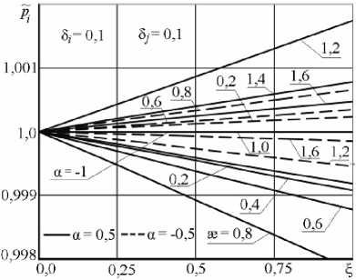
Рис. 6. Оценки собственной частоты при различных значениях ξ и æ

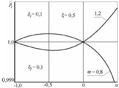
Рис. 7. Оценки собственной частоты в зависимости от параметра α

• Fig. 6.    Estimates of the natural frequency at different values of ξ and æ

• Fig. 7.    Estimates of the natural frequency as the function of the parameter α

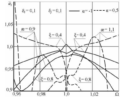
Рис. 8. Оценки обобщённой массы при различных величинах ξ и æ

Fig 8. Estimates of the generalized mass at different magnitudes of ξ and æ

When determining the natural frequency using the condition λ = 0 in the case L = N , it was found that the relative natural frequency p͂i = 1 when æ = 1 и p͂ i < 1 when æ < 1. Here, with L < N , the ratio of the natural frequency of the mode found by λ crossing zero ( p i^* ) to the exact value of this frequency ( p i ) depends on the size and sign of parameter α. When α = –1 (combining symmetric and antisymmetric modes) and damping of the modes is less than 0.15, p i^* practically matches pi regardless of æ and ξ. When –1 < α < 0, the relationships between p i^* and p i for æ < 1 and æ > 1 are opposite to those for the case L = N .

The value of α has the greatest impact on the accuracy of determining the generalized mass. Comparing results for L < N with calculations for L = N , we see that if the system has symmetric and antisymmetric modes, the generalized mass is determined more accurately using formula (15) than (14). With symmetry broken, the errors in mass calculation sharply increase near the natural frequency of the mode. For example, with α = 0.5; 0.9 ≤ æ ≤ 1.1 and ξ ≥ 0.8, the errors a_i exceed 10% if the frequency of forced vibrations differs from the natural frequency by less than 0.1%. With æ = 0.975 and ξ ≥ 0.1, there are no frequencies near Ω = 1 where a͂_i > 0.9.

Conclusion

The results of studies on errors in determining generalized dynamic characteristics in modal tests, used for correcting calculation models of AC type (1), are presented. It was established that the reliability of experimental evaluation of natural frequencies serves as a basis to consider them as parameters of the target function for correcting the stiffness matrix of the calculation model. At the same time, correcting the inertia matrix, developed during the design stage of the AC, is not advisable due to large errors in the estimates of generalized masses. This approach to solving the problem of correcting calculation dynamic models of structures is followed, for example, in works [19; 20].

Correction of the calculation inertia matrix can be sufficiently carried out by monitoring changes in the mass-inertia characteristics of the AC during its creation and operation. Consideration of these changes is reflected in the relevant acts and certificates.