Интеграция машинного обучения и алгоритмов пчел с многоагентными системами для динамической задачи маршрутизации транспортных средств с временными окнами

DOI:

Combinatorial optimization problems like the DVRPPDTW are central to operations research involving the optimal allocation of resource that meets demand. These problems are complex due to the exponential growing of solutions and the need to handle real-time changes such as changing delivery request and time windows which traditional methods struggle to tackle [1]. MHs including Genetic Algorithms (GA) [2], Ant Colony Optimization (ACO) [3], and BA [4] are effective tools for finding high quality solutions in reasonable time. However, their performance highly depends on parameter settings configuration, exploration and exploitation in dynamic environments such as DVRPPDTW [5]. To improve adaptability and performance of MHs the ML has been integrated with MHs. Supervised techniques like RF allow for dynamic prediction of optimal parameters which enhancing MHs ability to adapt to different problem instances and improving solution quality in real-time scenarios [6].

This paper present LBA by integrating ML into BA which further enhanced by MAS for decentralized decision making. RF is used for parameter tuning while MAS allows each vehicle to act as independent agent making real-time adaptions based on local information. This combination ensures robustness and efficiency in optimizing routes within DVRPPDTW [7]. This study explores the integration of ML and MHs to improve vehicle routing in dynamic environments. Previous work has demonstrated that combining supervised and reinforcement learning can improve customer service efficiency by 12% in high-density areas but challenges remain with dependence on historical data and computational demands [8]. A hybrid ML and combinatorial optimization method excelled in same day deliveries but was constrained by fleet size assumptions [9].

Dynamic routing for simultaneous delivery and pickup has produced mixed results. While the Golden Ball Algorithm struggled with scalability [10] and memetic algorithms showed potential despite facing challenges with scaling to larger instances [11], [12], [13]. A novel egrocery routing framework improved efficiency by 30%, though larger-scale applicability needs further study [14]. GA and ACO demonstrated effective real-time adaptation but require enhancements to handle higher dynamism and larger instances [15], [16]. The CLARITY method showed promise in combining clustering and evolutionary algorithms but needs further exploration in larger environments [17]. The results confirm the effectiveness of the proposed approach in reducing travel distance and increasing the number of deliveries, particularly in dynamic environments. The algorithm consistently outperforms existing methods enhancing adaptability and ensuring efficiency and reliability under various operational conditions.

Problem definition

The DVRPPDTW is complex problem within the field of logistics and transportation. This problem includes routing fleet of vehicles in dynamic way to provide services to a set of pickup and delivery requests so each with specific time windows during at which they must be

completed. Unlike static vehicle routing problems DVRPPDTW requires real-time decision making continuously as new requests and changing conditions[14]. The objective is to minimize the total travel distance when ensuring that all pickup and deliveries are completed within their time windows and vehicle capacity constraints. DVRPPDTW is important in industries like e-commerce and courier services where efficiency and rapid interaction are important to meet the customer’s demands in dynamic environments. Solving DVRPPDTW in effective way can lead to significant cost savings and service improvements. The problem formulation is as follow:

Sets:

• V : Set of vehicles.

• C :    Set of customers.

• D :    Set of delivery locations.

P : Set of pickup locations.

T : Set of time windows.

K : Set of vehicle capacities.

Decision Variables:

C ij : Cost (distance/time) of traveling from location i to location j.

d j : Demand at location i (either delivery or pickup).

q_v : Capacity of vehicle v .

t l^tart , t i^nd : Start and end of the time window for service at location i.

M : A large constant (used for linearization).

X_i j _v : Binary variable, 1 if vehicle v travels directly from location i to j, 0 otherwise.

y_iv : Binary variable, 1 if vehicle v serves location i, 0 otherwise.

z_iv : Time when vehicle v starts service at location i.

u_iv : Load of vehicle v after serving location i.

min

2° X ° X v=V iECUD jECUD

^C ij ^X ijv

2 Xijv- iECUD

X X jiv = 0 jECUD

VI ECUD,Vv EV

ulv + dj. Xjlv < qv     Vi E C U D,Vv E V(3)

uiv >0  Vi EP,Vv EV(4)

ziv + tij < zjv + M . (1 - Xijv) Vi,j ECUD,Vv EV(5)

t?tart < ziv < t4nd    Vi ECUD,Vv EV(6)

и Vi EP, Vj ED,Vv EV(7)

,Vv EV(8)

, Vv E V(9)

Vi,j ECUD(10)

Vk,V(i,j,l) E CU D(11)

^z i

< z.

- zjv

2 y^=1

iECUD

2 у» = 1

jECUD

2xuv< 1

vEV

X

<

The objective function aims to minimize the total distance traveled by the fleet in equation (1). The flow conservation constraint (2) ensures that each vehicle maintains route continuity. Capacity constraints (3) and (4) ensure that the load carried by each vehicle does not exceed its capacity at any point during the route. Time window constraints (5) and (6) enforce that all services, including pickups and deliveries, are performed within the specified time windows. The pickup before delivery constraint (7) ensures that pickups occur before their corresponding deliveries. Depot constraints (8) and (9) ensure that all routes start and end at the depot. Collaborative constraint (10) for fleet ensures that each customer served once by only one vehicle. The route continuity and real-time adaptation in constraint (11) allow the routing plan to be updated based on real-time information to ensure that the fleet can adapt to changes occur[14].

METHODS

This section presents the details of the methodology to solve the DVRPPDTW by integrate the BA, MAS, and RF. The proposed algorithm in figure 1 utilizes these methods to optimize

vehicle routes dynamically when considering time windows, and pickup and delivery constraints and shared fleet capacity. The following subsections describes the LBA.

Bee Algorithm

The BA is nature inspired optimization algorithm that mimic the foraging behavior of honeybees[18]. It is known to be effective for solving optimization problems by balancing exploration and exploitation. In the context of DVRPPDTW the BA used to find optimal routes for vehicles which minimize the total travel distance and meet time window constraints. The steps of BA:

• 1.    Initialization : Set the parameters values and generate initial solution (population) for scout bees at which each one representing potential vehicle route.

• 2.    Fitness Evaluation : Evaluate the fitness of the bees based on total travel distance and time

• 3.    Selection of Best Sites : Sort bees based on fitness and select the best performing bees (elite sites) for more intensive search.

• 4.    Neighborhood Search : Recruit forager bees to explore around the best sites which refines the potential solutions.

• 5.    Scout Bees : Assign remaining bees to explore new areas of the solution space randomly.

• 6.    Iteration and Update : Combine the best solutions from neighborhood searches and scouts, update the population, and repeat until convergence or maximum iterations are reached.

window constraints.

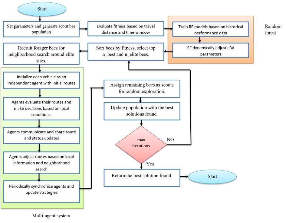
Figure 1. The flow process of the LBA.

Algorithm 1: Bee algorithm

• 1.    Initialize scout bee population randomly.

• 2.    Evaluate fitness of each scout bee.

• 3.    For iteration = 1 to max_iterations do:

• 4.    Sort bees by fitness.

• 5.    Select top n_best bees as best sites.

• 6.    Designate n_elite bees from n_best for intensive search.

• 7.    For each elite site:

• 8.    Recruit forager bees for neighborhood exploration.

• 9.    For non-elite sites:

• 10.    Recruit fewer forager bees for neighborhood exploration.

• 11.    Assign remaining bees as scouts for random exploration.

• 12.    Generate new random solutions for scout bees.

• 13.    Update population with the best solutions found.

• 14.    If stopping criteria met, exit loop.

• 15.    Return the best solution and its fitness value.

Multi-Agent Systems

The MAS enhance the capability of the BA by enabling decentralized decision-making and improving scalability. In MAS, each vehicle operates as an independent agent with the ability to make real-time decisions based on local information and collaborate with other agents [19]. This decentralized approach is particularly effective for handling the dynamic aspects of DVRPPDTW, such as real-time delivery requests and changes in vehicle status. The steps of MAS:

• 1    Agent Initialization : Set up each vehicle as an independent agent with an initial route and scout bees.

• 2    Local Decision-Making : Agents evaluate their routes and make decisions based on local conditions.

• 3    Agent Communication : Agents share route and status updates to coordinate efforts.

• 4    Dynamic Adjustment : Agents adjust routes based on local searches and information from others.

• 5    Global Coordination : Periodically synchronize to align with overall goals and update strategies.

Algorithm 2: Multi-Agent Systems

Inputs: n_scout, n_selected, n_elite, n_best, max_iterations, problem-specific parameters, initial scout bee population

Output: Optimized routes

• 1.    Initialize each vehicle as an independent agent

• 2.    Generate initial population of scout bees for each agent

• 3.    While (current_time < end_time):

• 4.    Each agent collects real-time data (new orders, status updates)

• 5.    Each agent evaluates its scout bees

• 6.    Agents communicate and share information

• 7.    Each agent dynamically adjusts parameters using local information

• 8.    Each agent performs local neighborhood search and random exploration

• 9.    Periodically synchronize agents

• 10.    Central coordinator collects performance metrics

• 11.    Return optimized routes

Random Forest for Parameter Tuning

The RF is employed to enhance the BA’s performance by dynamically tuning its parameters and selecting the most effective neighborhood exploration operators. RF models are trained using historical data to predict optimal parameter settings and operator choices, allowing the algorithm to adapt to different problem instances and improve overall performance [6]. The steps of RF for parameter tuning:

• 1    Data Collection : Run BA with varying parameters and operators, recording performance metrics.

• 2    Model Training : Train RF models to predict optimal parameters and operators based on historical performance data.

• 3    Prediction and Adjustment : Use RF predictions during BA execution to dynamically adjust parameters and choose the best operators.

Algorithm 3: Random Forest

Inputs: Historical data, initial scout bee population, training data for RF models

Output: Optimized routes, trained RF models

• 1.    Collect and preprocess historical data.

• 2.    Train RF models:

• a.    One model for parameter tuning.

• b.    One model for operator selection.

• 3.    Initialize BA parameters and scout bee population.

• 4.    While (stopping criteria not met):

• 5.    Evaluate and sort scout bees by fitness.

• 6.    Select and intensify search on top bees (elite sites).

• 7.    Perform neighborhood exploration for selected sites.

• 8.    Assign scouts for random exploration.

• 9.    Update population with best solutions.

• 10.    Use RF models to predict and adjust parameters and operators.

• 11.    Return the best solution found.

Experimental setup

The experiments were conducted on a laptop with an AMD Ryzen 7 5800H CPU and 16 GB of RAM using Python for implementation. The dataset, sourced from Küp's original publicly available paper, which represents the first documented use of real-time data to tackle this problem to the best of our knowledge, includes detailed attributes for solving the vehicle routing problem. Delivery attributes such as deliveryId, location (latitude, longitude), timing (orderTime, serviceTime), and delivery windows (start and end times) are provided. Vehicle attributes include vehicleId, courierId, vehicleName, and capacity. The dataset also specifies operational hours and methods for calculating distances, enabling comprehensive route optimization based on timing, capacity, and distance.

RESULTS

The computational results of this work presented in this section. BA was utilized for the DVRPPDTW. The parameters are dynamically tuned using RF to enhance the algorithm performance. In table 1 RF was used to dynamically adjust these parameters ensuring the BA adapted effectively to different scenarios. This approach balanced exploration and exploitation leading to optimized routes and improved algorithm efficiency.

Table 1. Parameters values of BA.

Parameter	Description	Value	Role
n_scout	Number of scout bees	34	Generates initial random solutions across the search space.
n_selected	Number of selected bees	27	Chooses the best performing solutions for further exploration.
n_elite	Number of elite bees	11	Focuses search on the most promising solutions for intensive refinement.
n_best	Number of best sites	15	Concentrates the search effort on the best performing areas of the solution space.
max_iterations	Maximum number of iterations	376	Ensures that the algorithm stops after a predefined number of cycles, preventing excessive computation.

Table 2 compares the performance of three algorithms: Küp et al.’s algorithm [14], the proposed LBA, and the basic BA across various vehicle IDs focusing on metrics such as the number of deliveries in Market 1 (M1) and Market 2 (M2) as well as the total distance traveled. The LBA generally shows an improvement in the number of deliveries made in Market 1. For example vehicle ID 6 made one additional delivery compared to Küp’s approach indicating that the dynamic adjustment strategies in LBA are more effective in handling fluctuating delivery demands. This improvement suggests that LBA is better equipped to handle the dynamic nature of delivery requests. In Market 2 the LBA also demonstrates slight increases in delivery numbers for some vehicle IDs (e.g., Vehicle IDs 8 and 11) reinforcing its ability to manage varying delivery demands especially in high density areas. The total distance traveled by the vehicles is consistently lower with LBA compared to the other algorithms. For instance, vehicle ID 5 showed a reduction in total distance from 175217 with Küp’s algorithm to 174687 with LBA. This reduction while small demonstrates LBA’s efficiency in optimizing routes. Over large-scale operations these small improvements in distance can lead to significant cost savings in terms of fuel and time efficiency. The results suggest that LBA is more effective than both Küp’s algorithm and BA in reducing total travel distance and managing dynamic delivery requests. This indicates that the integration of ML techniques (as seen in LBA) provide actual benefit in optimizing complex routing problems. Although BA shows near performance to Küp’s algorithm the consistent performance of LBA across different vehicle IDs highlights its superior adaptability and efficiency in dynamic environments.

Table 2. Comparison results of Küp’ algorithm, LBA, and BA.

< У О	«3 ^ в в с. в с.	2 р в «5 в г В rt-ф	Küp et al.’s algorithm			LBA			BA
			О 2 к Р 2, -S ^ в	О 2 к Р -S bJ	О rt- л	О 2 к Р © 2, в	О 2 к Р © 2, bJ	rt-в О rt- л	О 2 к Р в	О 2 к Р © 2, bJ	rt-в О rt- л
0	47	0	0	0	166694	0	0	166253	0	0	167434
1	50	0	0	0	170583	0	0	170843	0	0	171240
2	50	0	0	0	146823	0	0	146337	0	0	147719
3	49	0	0	0	162635	0	0	163061	0	0	163521
4	50	0	0	0	169870	0	0	169589	0	0	170767
5	40	1	10	0	175217	8	0	174687	7	0	175881
6	15	2	9	25	169575	10	26	169034	5	18	170269
7	47	0	0	0	153759	0	0	153988	0	0	154423

8	29	1	21	0	167572	23	0	167085	14	0	168316
9	50	0	0	0	162972	0	0	163159	0	0	163847
10	36	1	13	0	150875	11	0	150518	7	0	151584
11	0	2	53	22	208333	56	19	207923	41	15	208984
12	53	0	0	0	180110	0	0	180527	0	0	180933
13	39	1	10	0	155523	14	0	155006	6	0	156156
14	49	0	0	0	179146	0	0	179483	0	0	179939
15	52	0	0	0	169696	0	0	169469	0	0	170566
16	45	1	0	4	153758	0	3	153470	0	0	154428
17	53	0	0	0	170857	0	0	170514	0	0	171517
18	34	1	12	0	143507	15	0	142838	4	0	144388

Performance analysis

Table 3 summarizes the algorithm’s performance across various vehicle IDs focusing on key metrics like standard deviation (SD), Mean, SD/Mean Ratio, minimum time (Min Time), and average time (Avg Time) over 30 runs. The low SD/Mean Ratios such as 1.3% for Vehicle ID 0 and 1.1% for Vehicle ID 7 for instance indicate high reliability with least variability around the mean. The Min Time and Avg Time metrics like 9.28 and 14.80 seconds for vehicle ID 3 demonstrate the efficiency of the proposed algorithm in delivering optimized routes. This combination of less variability and high efficiency emphasizes the suitability of the algorithm for real-time dynamic routing changes where rapid decision making is important. These metrics show that the algorithm is efficient and reliable making it a strong candidate for dynamic vehicle routing problems.

Table 3. Descriptive metrics values of our algorithm performance.

Vehicle ID	SD	Mean	SD/Mean Ratio	Min Time	Avg Time
0	2411.55	173651.65	1.3%	6.51	12.81
1	3191.77	174107.97	1.8%	8.11	10.41
2	2980.80	150831.16	1.9&	7.27	12.62
3	2626.78	166532.88	1.5%	9.28	14.80
4	2927.46	172801.89	1.6%	6.28	13.70
5	2272.39	178582.18	1.2%	4.92	8.84
6	2518.33	172435.44	1.4%	11.65	17.80
7	1818.37	157519.41	1.1%	8.08	11.57
8	2462.74	170053.38	1.4%	5.44	14.16
9	2419.97	166791.45	1.4%	8.07	9.04
10	2247.21	154160.04	1.4%	14.87	22.76
11	3201.72	210594.35	1.5%	24.05	59.49
12	2256.78	184193.52	1.2%	43.13	129.68
13	3566.36	158648.00	2.2%	25.31	60.66
14	3042.14	182090.55	1.6%	23.36	60.40

15	2586.65	173345.14	1.4%	23.87	59.88
16	2413.86	157136.32	1.5%	23.53	62.64
17	2241.85	167181.16	1.3%	24.78	64.27
18	1796.94	146307.83	1.2%	23.56	57.91

Table 4. Wilcoxon test of MAS approach and non-MAS approach.

Vehicle ID	P-value	Vehicle ID	P-value
0	0.03818	10	0.0113
1	0.04236	11	0.04872
2	0.04838	12	0.03085
3	0.02894	13	0.02361
4	0.03387	14	0.05978
5	0.01706	15	0.04263
6	0.05384	16	0.02801
7	0.04611	17	0.02894
8	0.04161	18	0.03922
9	0.05712

The Wilcoxon test results in Table 4 demonstrate that the LBA approach significantly outperforms the BA approach for most vehicle IDs, with p-values below 0.05 in the majority of cases. This indicates that LBA generally provides a meaningful performance improvement, likely due to its real-time adaptability and collaborative route optimization. However, for a few vehicles (IDs 6, 9, and 14), the differences were not statistically significant, suggesting that the benefits of LBA may vary depending on specific scenarios.

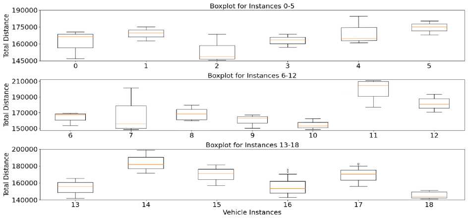
Figure 2. Box plot representation of vehicles’ performance from 0 to 18.

A box plot visually displays data distribution using a five-number summary: minimum, first quartile (Q1), median, third quartile (Q3), and maximum. The box represents the interquartile range (IQR), containing 50% of the data, with the median inside. The whiskers extend to the minimum and maximum values, excluding outliers, which are shown as individual points. Figure 2 visually represents the algorithm’s performance across different vehicle IDs using box plots, highlighting the distribution of results over 30 runs. The tight clustering of data, particularly for Vehicle IDs 1,3,5,6,8,9,10,12,13, and 18 shows that the algorithm consistently produces results better than average, with minimal outliers. Even in cases like Vehicle IDs 0,7,2,16, and 17 where some variability exists, the overall narrow distribution reflects the algorithm’s reliability. The few outliers suggest challenging conditions, but the algorithm's consistent performance across most runs underscores its adaptability in dynamic environments.

DISCUSSION

The comparative analysis demonstrates that LBA significantly outperforms Küp’s approach in several key areas particularly in dynamic vehicle routing scenarios. One of the primary strengths of LBA is its dynamic adaptability. The algorithm’s ability to incorporate real-time data and adjust routes based on fluctuating demands as evidenced by the performance in Markets 1 and 2 ensure that it maintains high service levels even as delivery requests change rapidly. Additionally, the distance reduction remains important advantage as they are consistent through most vehicle IDs. This consistency is essential as even small improvements in large scale operations can lead to significant cost saving in fuel consumption and time efficiency. The improvements suggests that LBA can optimize routes in effective way through different scenarios making it a worthy tool for logistics operations. However, two limitations were observed in the study. First the scalability, while LBA performed well in the tested instances but its ability to handle more complex and larger scale environments remains uncertain. Second the effectiveness of LBA is highly dependent on specific parameter tuning which can be a limitation. The performance of the algorithm may vary significantly based on the chosen parameters and finding the right balance can require additional effort.

CONCLUSION

The proposed algorithm enhances the optimization of dynamic vehicle routing problems significantly by integrating ML with BA and MAS. The hybrid method offers robust solution of real-time route modifications tackling the complexities of the DVRPPDTW in effective way. By employing RF regression for parameter tuning and MAS for enabling decentralized decision making ensures efficient and adaptable performance across various scenarios. The impact of this approach is evident in its ability to reduce total travel distance and improve delivery efficiency directly benefiting logistics operations. The performance analysis demonstrate that the algorithm consistently outperforms existing method offering scalable and reliable solution for dynamic environments. The results confirm the approach’s effectiveness by reducing the total travel distance by about 5% and increased the number of deliveries by about 12% making it a valuable tool for addressing real-world vehicle routing challenges.