Iterative Models for Calculating Magnetic and Electric Circuits in Electrical Machines

Цитирование: Жакатаев Т. А. Итерационные модели для расчета магнитных и электрических цепей в электрических машинах / Т. А. Жакатаев // Журн. Сиб. федер. ун‑та. Техника и технологии, 2026, 19(5). С. 668–681. EDN: AGKSUH known fact. It should not be, and is not logical, to try to embrace in one review so great a variety of this material.

Most likely this is a function of AI and Big Date, to process very polynomial publications.

One of the important points in the calculation and design of new machines is the methodology for calculating magnetic circuits. And the associated methodology for calculating electric circuits. This task has especially high significance for our country. Because we belong to the group of developing countries. In the sense that both during our time within the Soviet Union and after it, we engaged very little in the development and creation of new machines and new technologies. For the most part, we went along the path of simple consumers and buyers. That is, all the main machinery, machines, instruments, and equipment were brought to us from outside, from other countries. We were mere purchasers and users of ready‑made technical equipment. However, time dictates us its new laws and rules. Our youth, who have higher technical education, have grown in number and have become stronger in quality. Therefore, the young generation of engineers is ready to begin the development and creation of new machines, technologies, and equipment. And any new undertakings and projects, as is known, need scientific and theoretical support and technical provision. We hope for the help and support of engineers and scientists from all over the world.

Taking the above into account, our present work is devoted to the issue of developing and implementing new iterative schemes and models for the calculation of magnetic and electric circuits in the most diverse types and designs of electrical machines.

Which are available in simple manual programming mode. And they can be implemented on the simplest PCs. In other words, our work and our results are intended for engineers – developers of new electrical machines, structures and equipment. In the new conditions of technological progress for mass and widespread use.

We have solved a problem of analysis in the theory of calculating magnetic circuits [1–5] using automation of the computational algorithm. Based on numerical computer calculations. According to it, for a given magnetizing force F = Iw , the induced induction B_i is calculated over all sections of a complex nonlinear magnetic circuit and B A in the air gap. In the scientific and educational literature, this problem is also called the inverse problem, or also the second Kirchhoff’s law for a contour of a magnetic circuit [1–5].

Features of interpolation formulas application in calculation of magnetic characteristics of various circuits are shown. Clarifications were made when using them.

Theoretical Solution and Results

Most electrical machines (abbreviated EM) are reversible. They can operate both as generators and as motors.

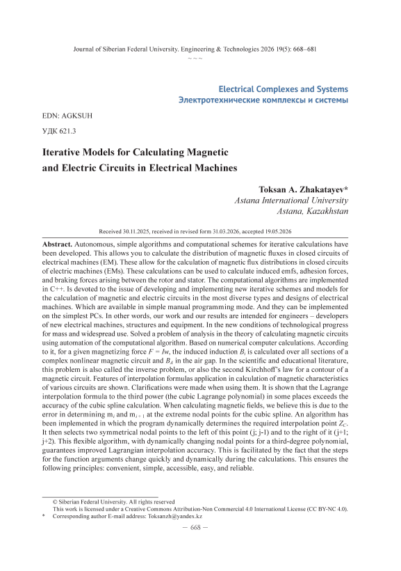
To compose and test a new calculation model, we considered a simplified diagram of an electrical machine [1–7], presented in Fig. 1.

We endeavored to come as close as possible to the size of some actually existing generator. To this end, the initial working drawing was executed on a large sheet of drawing paper. In order to see and understand the real dimensions of a real electrical machine, abbreviated EM. Therefore, the outer diameter of the housing amounted to 352 mm. The length of the housing is 400 mm. The slots on the stator were made wider and deeper to place many windings, so that there would be many conductors on the stator. As a result, the transverse dimension of the stator tooth became smaller,

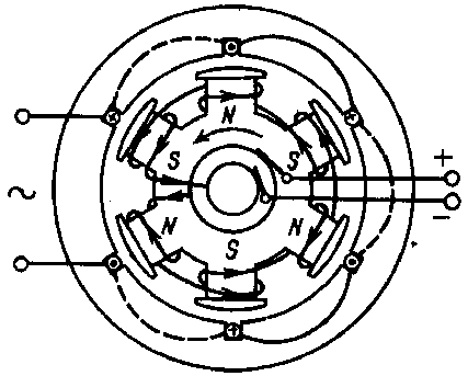
Fig. 1. General diagram of an electric reversible ma‑ chine [1, 3, 7]

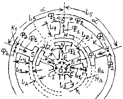
Fig. 2. Detailed scheme of circulation of the magnetic field vector in the rotor and stator in an EM cross‑section

and it became almost equal in width to the size of the rotor tooth. In turn, the teeth on the rotor were increased in cross‑section, and the diameter of the very post of the tooth was decreased. So that in the space between neighboring teeth of the stator and rotor, as many as possible windings of copper wires could be placed. Thus, we were able to wind 200 turns of wire of 3 mm diameter on one rotor tooth. On one stator tooth, we wound 240 turns of wire of 4 mm diameter. These are otherwise called windings.

Thus we considered specifically the following type of EM in cross‑section, which is shown in Fig. 2.

When calculating and designing an EM, an important point is the use of the nonlinear graph of dependence B = f ( H ) for the magnetic core [1–6], Figure 3. In which the different numerals 1–4 refer to different grades of electrical steel: E‑11, E‑31, E‑42, E‑45 [7–12].

Currently, all design calculations are carried out on a PC using a programmable algorithmic language. The design works can include almost the entire range of changes of H, A/m.

Moreover, the specific required values can be any, that is, arbitrary. Therefore, the most correct method is that the values of B = f ( H ) should be tabulated. Then the necessary number of discrete values of B_i = f ( H_i ) should be entered into the computational program. With a certain step. For arbitrary values of H ≠ H_i (which differ from these support points) all computations are carried out on the basis of using some interpolation formula.

In composing the computational program, we used two interpolation formulas: 1) interpolation by cubic splines; 2) the Lagrange interpolation formula, also cubic, that is, this too is a third‑degree polynomial.

• 2.1.    Solution for spline interpolation.

As a working formula we chose the following popular formula [13–25]:

fi+1 +

(x_i+1 -%)²(2(x -Xi) +h_x) (x - Xi)²(2(x_[+1 - x) + h_x)

Sx =--------------74-------------ft ^--74-------------- hx                             hx

where mt = S^xJ , m_i+1 = 5з(^+1) – are the derivatives of formula (1) at points x_i and x_{i +1}; f_i , f_{i +1} – are the values of the desired function at these same points, and h x is the step along the x‑coordinate. For an approximate calculation of m_i , the following formulas are given in [13–19]:

_4A-/₂-3/₀ ^m° 2h_x

_ 3f_N Wn-! + f_N_₂

™N~ ж

where mi = fi^' are the values of the derivatives at the nodal points.

Fig. 3. Magnetization curve of electrical steels of various grades [1, 3, 7]

We developed and composed our own calculation program in C++, which performs computations by formulas (1) and (2).

Formulas (2) represent a simplified variant. As our computational practice has shown, nevertheless, for engineering calculations, it is quite suitable. Only in some cases did the error amount to 0.95 %.

In books, there are also schemes for calculating the coefficients m_i through second‑order difference schemes [13–25]. This is the so‑called scheme for calculating mi via the sweep (Thomas) formulas. In our subsequent research, we plan to carry out calculations on the basis of the cubic splines (1). m_i will be computed by the three‑point sweep formulas [13–15, 16, 25]. For three‑point difference equations for m_i . We are speaking only about calculations in application to magnetic and electric schemes, as we noted at the beginning of this article.

• 2.2.    Application of Lagrange interpolation formulas.

The Lagrange interpolation formulas for one‑dimensional, two‑dimensional and three‑ dimensional interpolation are known to have the forms [13–15, 16, 25]

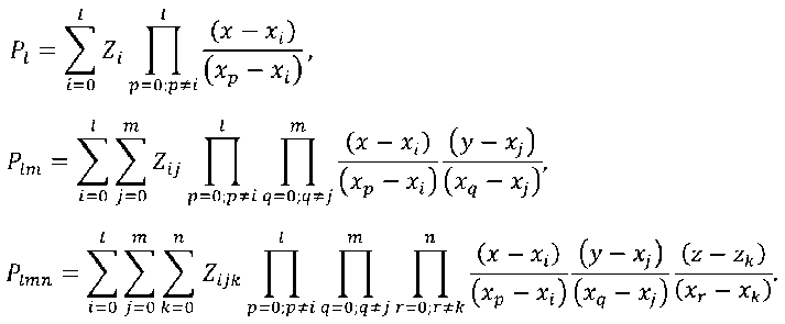
When composing the calculation program in C++ according to formula (4), we applied the method of successive iteration along the first coordinate (j) with the second coordinate (i) “frozen” and fixed. We explain the said by Figure 4.

That is, at first we take our position (stand) on the coordinate line i –1 . We apply one‑dimensional Lagrange interpolation. Using points 1, 2, 3, 4, we calculate point z ₁ More precisely, we calculate the value of the two‑dimensional function f ( z ₁) at this point. Next, we move to coordinate line i . We use the values of function f_{i ,} j at points 5, 6, 7 and 8. We calculate the value of function f ( z ₂) at point z ₂. Next, we move to coordinate line i + 1. We use the values of function f_{i ,} j at points 9, 10, 11 and 12. We calculate the value of function f ( z ₃) at point z ₃. Similarly, we find f ( z ₄) for point z ₄.

Now we know four values of f i for four points z i . We once again (that is, reapply) one‑dimensional Lagrange interpolation for these four points z _i and calculate the value of f _c for point z_c. Thus, we have calculated two‑dimensional Lagrange interpolation. The four points for each coordinate were deliberately chosen. In this case, the Lagrange interpolation formula becomes a cubic polynomial. With the correct choice of density (frequency) of nodal points, a third‑degree polynomial describes all experimental curves and graphs with sufficient accuracy. With any steepness and curvature that can be observed in engineering practice.

Computational practice has shown that when using polynomials of degree 3 or less, there are no oscillations or “spikes” in the calculated point values outside the permissible range. This means that sudden spikes and unnecessary jumps do not occur. Lagrange polynomials of lower degrees are no different from spline functions. In terms of calculation accuracy and smoothness requirements,

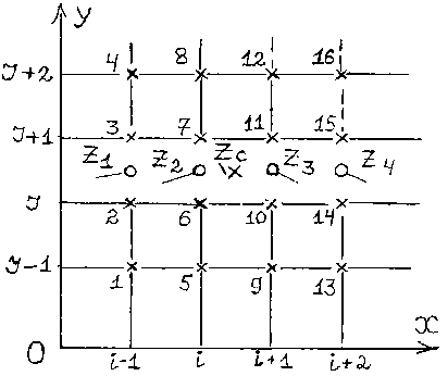
Fig. 4. Schema of a grid stencil on the plane for two‑dimensional iteration functions in the interpolation domain can be even better. We implemented an algorithm in which the program dynamically determines the required interpolation point ZC. It then selects two symmetrical nodal points to the left of it (j; j‑1) and to the right of it (j+1; j+2). This flexible algorithm, with dynamically changing nodal points for a third‑degree polynomial, guarantees improved Lagrange interpolation accuracy. This is facilitated by the fact that the steps along the function arguments change quickly and dynamically during the calculations. This ensures the following principles: convenient, simple, accessible, easy, and reliable.

It’s clear that we didn’t originate this solution: to ensure that the x coordinate (variation i ) is fixed when moving along the y coordinate (variation j ). This is noted, for example, in [14–19]. However, it’s one thing to merely sketch this out, just briefly, superficially. Just as an idea. What we’ve accomplished in this paper is quite another. Specifically, we’ve described this working algorithm in detail, based on dotted line diagram 4. Such a detailed, simple, and clear description of this process is necessary and useful for various programmers, calculators, engineers, and designers. This is so they can independently develop and compile correct computational algorithms and programs. The ability to present material clearly, intelligibly and completely is a great and useful thing.

Let’s now move on to examining three‑dimensional interpolation using formula (5). We add another axis, OZ, to Figure 4. It’s not visible in Figure 4 because it’s perpendicular to the plane of the drawing. We must select four slices, four planes, along this axis. They are parallel to this initial OXY plane. Four points z _{c, k} must be calculated on these four planes. More precisely, four values of the function f ( z c, k ), k = 1,2,3,4 – must be calculated. Finally, a single value, f ( w ), is calculated from these values – this is the unknown value of the function at the interpolated point w in three‑dimensional space [x, y, z]. In this case, one‑dimensional Lagrange interpolation was used when iterating (“ran”) through the values of k.

What is the purpose of iteration? By repeatedly repeating the calculations using one‑dimensional interpolation, we arrive at multidimensional interpolation based on iteration. That is, we perform iterative runs as ( i , j , k ) changes.

The world of engineering physics and engineering technologies is limited primarily to three‑ dimensional functions: density, volume, torque, and so on. Therefore, we limited our consideration to three‑dimensional interpolation using both Lagrangian and cubic spline methods.

Complete proofs of formulas (4) and (5) are very rare. Of all the books listed in the bibliography, we found a complete proof in only one source [17]. Engineers are also typically very inquisitive; they also want to know any theory in its entirety and depth.

• 2.3.    Iterative computations of magnetic fluxes in EM contours.

Consider Figure 2. Circuits OJKO and OJK ₁ O are symmetrical. In them, the magnetic fluxes Ф i – are also mirror‑symmetrical. Due to the complete symmetry of all six circuits of this EM, we show detailed calculations for only one circuit. Therefore, the magnetic driving force (mmf) of a single closed loop has the form

F = 2( H 1 L 1 + H A L A + H 2 L 2 + H 3 L 3 + H 4 L 4 ) + H 5 L 5 + H 10 L 10

where F = wI , w – is the number of turns in the winding, L ₁₀ = s ( DE ) = s ( FE ) [ m ], H [А/м], L [м], F and I is the current [A].

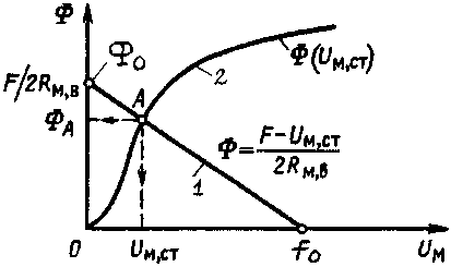
Fig. 5. Diagram explaining the iterative calculations of nonlinear magnetic fluxes in closed loops [1–6]

Further calculations are based on an iterative scheme, which is very well explained in Figure 5 from [1–6].

г la .                   . ..

Here, Фо —       , ^м,в ^— с – is the magnetic resistance of the air gap.

^^м,в' Fo^

During the iteration, the calculation program “moves” from point Ф 0 to point F 0 with a certain

Fo - Фо .           .      .             ..

step: hp —          . During the iteration, Ф h, i is constantly compared with the values of Ф( U м, ст )

,, along curve line 2 (OAФ). The values of Фh, i relate to the straight line 1 (Ф0 – F0), Figure 5. When the specified accuracy limit is reached, the calculations are stopped and the results are displayed. This is how the value of the magnetic flux in the EM air gap is calculated. At point A, the difference between Фh, i and Ф(Uм, ст) will be zero or very small. The proximity limit is specified. Point A is the air gap. The air gap is the space between the rotor and stator teeth. In our test calculations, LA = 1.3 mm.

Results: with a rotor winding current of I = 2 A , B A = 0.166 T ; I = 3 A , B A = 0.25 T . And this is when the current is only in the rotor winding. If additional current is applied to the stator winding with the same magnetic field orientation, the B A value can double. If the stator winding is connected in antiphase to the rotor, the B A value will decrease by almost half.

Why is the air gap magnetic field induction value B _A so important to know? The answer is that it can be used to calculate the induced e.m.f. In the stator winding, when the EM operates in generator mode [1–12]

E_s = 4.44/₁w₂O_a, (6)

where f 1 is the rotor speed, Hz, w 2 is the number of turns (windings) on one stator tooth, Ф А = B A S A .

As proof that we can indeed compose logical and dynamic algorithms and write computational programs ourselves, we present two small pieces, two subroutines in C++. These are part of the programs we have written. We write such programs ourselves, never using ready‑made templates or ready‑made algorithms. We have never used prompts from IT systems; AI is foreign to us and we do not use it. We are happy that we can work independently. From the very beginning, from scratch, from the very beginning, we can compose computational algorithms and program everything ourselves. We have more than 45 years of scientific and teaching experience.

/* subroutine for computing B for the air gap */

#include

#include

#include

#include using namespace std; int main() float const pi=3.14159;

float l1=75e‑3, l2=6e‑3, l3=l2, lvoz = 1.3e‑3, l4=61e‑3, l5=(pi/3)*172e‑3, l10=22e‑3;

float miuo = 4 * 3.14159e‑7, miugel = 5000.0, rvoz=99e‑3, alfavoz = 25*2*pi/180;

float avoz=alfavoz*rvoz, l2obsh=400e‑3 /* overall length */, ma=miuo*miugel, svoz=avoz*400e‑3;

float lobsh= 2*(l1+l2+l3+l4+lvoz)+l5+l10;

printf (“\n svoz=%10.3f”, svoz);

printf (“\n l5=%10.3f”, l5);

int n1=200, n2=240, ti1 = 3; /* xxxxx */ float fm1max=ti1*n1*2, rmvoz=lvoz/(miuo*svoz), fbmax=fm1max/(2*rmvoz), k1=fbmax/fm1max;

float kiter = 0.57, hxf=kiter*fm1max, ay=hxf*k1, fteki= fbmax‑ay;

float s1=12*400e‑6, s2=avoz*400e‑3, s3=avoz*400e‑3, s4=12*400e‑6, s5=8*400e‑

• 6, s10=15*400e‑6;

float h1=fteki*l1/(s1*ma), h2=fteki*l2/(s2*ma), hvoz=fteki*lvoz/(svoz*miuo);

float h3=fteki*l3/(ma*s3), h4= fteki*l4/(ma*s4), h5=fteki*l5/(ma*s5), h10=fteki*l10/(ma*s10);

float hobsh= 2*(h1+h2+h3+h4+hvoz)+h5+h10, bvoz=fteki/(svoz);

printf (“\n hobsh=%16.4f, hxf=%16.4f”, hobsh, hxf);

printf (“\n fteki=%16.4f, bvoz=%16.4f”, fteki, bvoz);

printf (“\n\n END RUN “);

getch();

return 0;

} /* end of subroutine */

/* Subroutine for computing one‑dimensional Lagrange interpolation */

#include

#include

#include

#include using namespace std; int main() { float yf, yf1, z1, z2, z3, z4, z5, z6, z11, z12, z13, z14, sf1, sf2, sf3;

int i, i1, i2, i3, i4, i5, i6, i7, i8, j, j1, j2, j3, j4, j5, j6, j7, j8;

float fx1[4][4] = {{3.0,7.0,11.0,15.0}, {5.0,9.0,13.0,17.0}, {7.0,11.0,15.0,19.0}, {9.0,13.0,17.0,19.0}}; int x1[4] = {1,2,3,4}, y1[4]={1,3,5,7}, u[4]={1,3,5,7}, v[4]={1,3,5,7};

float x[4], y[4][4], fx2[4];

int hx1[15], xx3[15], xx1[15], xx2[15]; int x1x=4, y1y=4, k1, k2, a1, a2, a3, a4;

j=1; j5=j‑1; j6=j; j7 = j+2;

for (i1 = j5; i1 <= j7; i1++) { yf=0.0;

for (i2=j5; i2<=j7; i2++) { z11=1.0; z12=1.0;

for (j2=j5; j2<=j7; j2++)

{ if (j2!= i2) { a1 = x1x – u[j2]; a2 = u[i2] – u[j2];

z11 = z11*a1;

z12 = z12*a2;

} } yf=yf+(z11/z12)*fx1[i1][i2];

} fx2[i1]=yf;

printf (“\n fx2[i1]=%10.3f”, yf);

} yf1=0.0;

for (i3=j5; i3<=j7; i3++) { z13=1.0; z14=1.0;

for (j3 = j5; j3<=j7; j3++)

{ if (j3!=i3) { a3 = y1y – v[j3]; a4 = v[i3]‑v[j3]; z13 = z13*a3; z14 = z14*a4;

} } yf1 = yf1 + (z13/z14)*fx2[i3];

} sf3=yf1; printf (“\n sf3=%10.3f”, sf3);

/* printf (“\n xz =%8d, xx=%8d, j=%4d”, xz, xx, j);*/ printf (“\n\n END RUN “);

getch();

return 0;

}

/* end of subroutine */

Discussion

Our critics may say: when there is MATLAB, Mathcad, Ansys (and other similar ones), why write other new, “manual” programs for computing by Lagrange interpolation and by cubic splines? And perform iterative computations in the so‑called “manual” mode of programming in known languages. Is this not extra work?

Answer. Such powerful and mobile programming languages as C++, Fortran, QBasic64 possess a whole range of high merits and positive sides. These include: their accessibility, simplicity of debugging and operation, flexibility, mobility, and reliability. They do not require excessively powerful, very modern, and expensive computers. They can autonomously operate and be launched on many old and simple models of computers and laptops. Installation packages do not require large volumes of permanent and RAM, they are simple and reliable in operation. In general, convenient, simple, accessible, reliable, flexible, and mobile.

With the so‑called “manual” programming, it is simple, easy, and convenient to get inside any program code, to change the steps along spatial and temporal coordinates. To vary many parameters of the computational scheme in a wide desired range. To find out the computation errors along all spatial and temporal coordinates. Which, for example, in MATLAB, Mathcad, Maple, and others, is impossible to do quickly. That is, in them, “manual” programming is impossible to apply. “Manual” means when all the program code, all computational steps, and algorithms the engineer writes himself in detail, step by step. Relying upon and using, of course, already known and proven mathematical and physical formulas, calculation schemes, and models.

One can give an example from another field. For example, issues of heat transfer. In open access, there are always many reference books in which various reliable formulas are given for calculating Nusselt numbers Nu = (ad)/λ. For different regimes of flow of a liquid or gas. In such cases it is also easier and simpler to carry out calculations when, by a formula, the engineer himself composes a computational program for himself according to our demonstrated method of “manual” programming. In ready‑made, big and powerful computational packages (MATLAB, Mathcad, Maple, SolidWorks, Ansys and the like – now there are many of them in software service) the design engineer does not – 678 – see the internal working formulas, does not know the internal kitchen, does not know the internal computational technology. Figuratively speaking, he simply eats a ready‑made dish. While not knowing what it is made of, and not knowing the technology of preparing this food. Therefore, many researchers are adherents of “manual” programming. Mobile programming.

We can also consider an example from chess. Yes, computer chess programs play faster and more powerfully than a human. Thousands, and perhaps millions of game variants and combinational moves are loaded into them. But nevertheless, people (that is, humans) continue to play chess. New champions appear. Living people create new moves, new solutions, new combinations. The popularity of playing chess among living people only increases with each year. So too with manual programming. It will not “die”. It will only develop forward.

People are drawn to simple, accessible, free, reliable, and mobile technologies. The potentially numerous audience of consumers must and should include retirees who are alive and well. Alongside the great mass of working (active) engineers, bachelors, master’s students, doctoral students, and other categories of scientific and technical people who are working at the present time. A person must not be forbidden to think, dream, and create at any age. One must not set barriers and brakes in the way of creative work at any age. Let every person create and build at any time, at any age, when he has the opportunity. Working even at home. Let a person make an independent, feasible contribution to world science and technology – even with his small steps. Which he is capable of. This is where the principles and logic of humanism, goodness, and justice lie. The modern popular motto is this: science, technology, and research – to the broad masses of the people.

Therefore, our work is appropriate, very useful, and in demand for many specialists and production engineers. It contains new theoretical solutions, algorithms, and programs.

We will now discuss a new, previously unknown idea for using formula (6). This formula calculates the induced emf in the rotor winding. It is based on the value of magnetic induction B A in the air gap. When generators and motors are large, the mass of individual rotor teeth, together with the wires wound on them, can reach large (significant) values. For example, this can be not just a few kilograms, but tens of kilograms in weight. Rotational speeds and frequencies can also be significant. In such cases, the centrifugal force of inertia can be quite large, leading to tensile deformation. This, in turn, can lead to a reduction in the air space (air gap) between the rotor and stator teeth. It’s clear that these strains will be very small. From the perspective of the large geometric dimensions of the machine, this will seem insignificant. However, we must be aware that a change in the air space layer δ _A by even tenths of a millimeter can significantly alter the level of the induced, generated e.m.f.

Therefore, we assume that formula (6) can be applied to practically detect changes (or fluctuations) in δ A . This can be done by observing the generation of E s in the stator winding. If the rotor serves as an electromagnet, this will be possible.

Added to this is the problem of linear thermal expansion (elongation) of individual stator and rotor teeth, which occurs as a result of heating these bodies. These changes can be calculated using simple formulas taught in standard heat transfer courses. We are confident that engineers can solve this problem independently. However, these results also lead to a decrease in δ _A. Therefore, solving this problem is also important and relevant for engineers who design new electrical machines and mechanisms.

Conclusions

• 1.    Autonomous, simple algorithms and computational schemes for iterative calculations have been developed. They allow calculating the distributions of magnetic fluxes in closed contours of electrical machines (EM). Using them, one can compute induced emfs, adhesion, and braking forces arising between rotor and stator. The computational algorithms are implemented in C++. In manual programming mode. On simple and affordable computers. For mass and widespread use.

• 2.    It is shown that the Lagrange interpolation formula of the third degree (cubic Lagrange polynomial) in places surpasses in accuracy the results of calculation by a cubic spline. In calculating magnetic fields. In our opinion, this is related to the error of determining m_i and m_{i + 1} at extreme nodal points.

• 3.    An algorithm has been implemented in which the program dynamically determines the required interpolation point Z C . It then selects two symmetrical nodal points to the left of it (j; j‑1) and to the right of it (j+1; j+2). This flexible algorithm, with dynamically changing nodal points for a third‑ degree polynomial, is guaranteed to improve the accuracy of Lagrange interpolation. This is facilitated by the fact that the steps along the function arguments change quickly and dynamically during the calculations. Thus, the following principles are implemented: convenient, simple, accessible, easy, and reliable. Oscillations of the function between nodal points are eliminated, which earlier could occur in interpolation calculations when the number of working points exceeded five.