Квадратичная минимизация и максимизация

Consider an extremum problem of a quadratic function over a box D e Rⁿ : f ( x ) = Cx , x ) + ( d , x ) + q ^ max(min), x e D ,        (1.1)

where C is an n x n matrix, d , x e Rⁿ , and D is a box set of Rⁿ . Here ^,-^ denotes the scalar product of two vectors.

Quadratic programming plays an important role in mathematical programming. For example quadratic programming surve as auxiliary problems for nonlinear programming in its linearized problems or in optimization problems approximated by quadratic functions. Also this has many applications in science, technology, statistics and economics. Moreover, many combinatorial optimization problems are formulated as quadratic programming including integer programming, quadratic assignment problems, linear complementary problems and network flow problems [7]. There are a number of methods for solving problem (1.1) as convex problem such as the interior point methods, the projected gradient method, the conditional gradient method, the proximal algorithm, penalty methods, finite step algorithm and so on [1, 9, 13]. Then well known optimality condition for problem (1.1) is in Rockafellar [10]. Also, the quadratic maximization problem is known as «NP» problem. There are many methods [3, 11, 12] and algorithms devobed to solution of the quadratic maximization over convex sets.

The paper is organized as follows. In section 2 we consider quadratic convex maximization problem and apply global optimality condition [11] to this. We propose some finite algorithms by approximation of the level sets of the objective function with a finite number of points and solving linear programming as auxiliary problems. In section 3 we consider the quadratic minimization problem over box constraints and recall the gradient projection method for solving this problem. In the last section we present numerical solutions obtained by the proposed algorithms for quadratic maximization and minimization problems.

2.    Quadratic Convex Maximization Problem 2.1.    Problem Statement and Global Maximality Condition Consider the quadratic maximization problem.

f ( x ) = ( Cx , x ) + dd , x) + q ^ max, x e D ,            (2.1)

where C is a positive semidefinite (n x n) matrix, and D e Rⁿ is a box set of Rⁿ . A vector d e Rⁿ and a number q e R are given. Then optimality conditions [12] can be also applied by proving the following theorem.

Theorem 2.1 [12] Let z e D be such that f ' ( z ) * 0 . Then z is a solution of problem (2.1) if and only if

(f '( У ), x - y ) <  0 for all У e E f ₍ z ) ( f ) and x e D ,         (2.2)

where E c ^{( f} ) = { y e Rⁿ |^{f (} y ) = c } .

Proof. Necessity. Assume that z is a global maximizer of problem (2.1) and let y e E_{f (} z ) ( f ) and x e D . It is clear f '( y ) * 0. Then the convexity of f implies that

• ⁰ ^ ^{f ( x} ) ^{- f (} z ) = ^{f ( x} ) ^{- f (} y ) > { ^{f ,(} y ), ^{x -} y)

Suffciency. Suppose, on the contrary, that z is not a solution to problem (2.1); i.e., there exists an u e D such that f (u) > f (z). It is clear that the closed set Lf (z)(f) = {x e R | f (x) < f (z)} is convex. Since int Lf (z)(f) = 0 then there is the projection y of u on Lf(z)(f) such that IIy — ull = xeminf Jlx - ull x e Ef (z)(f )

Clearly,

|| y - u || >  0                                      (2.3)

holds because u ^ L_{f ( z} ) ( f ). Moreover, this y can be considered as a solution of the following convex minimization problem:

g ( x ) = -21 x — Ц |² ^ min, x e E f ( z ) ( f )

Applying the Lagrange method to this latter problem, we obtain the following optimality condition at the point y :

X >  0, x >  о, x + X >  о

Ч g ( У ) + X f ( у ) = 0                     (2.4)

X ( f ( У ) - f ( z ) ) = о

If X 0 = 0, then (2.4) implies that X >  0, f ( y ) = f ( z ) and f '( y ) = 0. Hence we conclude that z must be a global minimizer of f over Rⁿ , which contradicts the assumption in the theorem. If X = 0, then we have X ₀ >  0 and g ‘ ( y ) = y - u = 0 , which also contradicts (2.3). So, without loss of generality, we can set X ₀ = 1 and X >  0 in (2.4) to obtain

У - u + X f ( y ) = 0, X >  0, f ( У ) = f ( z )

From this we conclude that ( f '( y ), u - y ^ >  0 , which contradicts (2.2). This last contradiction implies that the assumption that z is not a solution of problem (2.1) must be false. This completes the proof.

Sometimes it is also useful reformulate Theorem 2.1 in the following form. Theorem 2.2 Let z e D and rank ( C ) ^ rank ( CI d‘ ). Then z is a solution of problem (2.1) if and only if

(f '( У ), x — y ) <  0 for all y e E f ( z ) ( f ) and x e D ,     (2.5)

where ( C | d^t ) is the extended matrix of the matrix C by the column d^t .

2.2.    Approximation of the Level Set

Furthermore, to construct a numerical method for solving problem (2.1) based on optimality conditions (2.2) we assume that C is a symmetric positive defined n x n matrix. Then problem (2.1) can be written as follows.

f ( x ) = Cx , x ) + ( d , x ^ + q ^ max, x e D ,       (2.6)

where D = { x e R n I a <  x <  b } , and a , b , d e Rⁿ , q e R .

Now introduce the definitions.

Definition       2.1. The set       E_{f ( z )}( f )       defined      by

Ef ( z ) ( f ) = { у e R n I f ( y ) = f ( z ) } is called the level set of f at z .

Definition 2.2. The set A m defined by A _z™ = { y\y ²,..., y^m I y e E_{f ( z} ) ( f ) } is called the approximation set to the level set E_{f ( z )}( f ) at the point z .

Note that a checking the optimality conditions (2.2) requires to solve linear programming problems:

(f'(У), x — y) ^ max, x e D for each y e Ef (z)(f). This is a hard problem. So we need to find an appropriate approximation set such that one could check the optimality conditions at a finite number of points.

The following lemma shows that finding a point on the level set of f ( x ) is computationally possible.

Lemma 2.1. Let a point z e D and a vector h e Rⁿ satisfy (f '( z ), h <  0. Then there exists a positive number a such that ^z + ^a h e E f ( z ) ^{( f} ).

Proof. Note that ^ Ch , h >  0, and

(2 Cz + d , h <  0                         ⁽ 2.8)

Construct a point y _a for a >  0 defined by y _a = z + a h .

Solve the equation f ( y _a ) = f ( z ) with respect to a . In fact, we have

( ^C y a , y a ) ⁺ ( ^d , y a ) ⁺ 9 = ^{f (} z )

or equivalently,

CC (z + ah), z + ah) + dd, z + ah) + q = (Cz, z) + dd, z) + q hich yields

(2 Cz + d , h) ^a =     (Ch , h

By (2.8), we have a >  0 and consequently, y ₅ e E_{f ( z} ) ( f ).

For each y ' e A m , i = 1,2,..., m solve the problem

(f ‘ ( У' ), x^ ^ max, x e D .                  (2.9)

Let u^J , j = 1,2,..., m be solutions of those problems which always exist due to their compact set D :

(f '( y ' ), u ' ) = max x e D< f '( y ' ), x ).                (2.10)

Refer to the problems generated by (2.9) as auxiliary problems of the

A zm . Define 9 _m as follows:

⁹ m = max ( ^{f ,(} y j ), u ' - y j) j = 1,2,..., m '                             /

The value of 9 _m is said to be the approximate global condition value. There are some properties of A_z^m and 9 _m .

Lemma 2.2. If for z e D there is a point yk e Az1 such that (f (yk), uk - yk^ > 0Then f (Uk ) > f (z)

holds, where u^{k e} D satisfies ( ^f '( y^k ), u^k ) = max( ^f '( y^k ), x)

x e D

Proof. By the definition of uk , we have max (f,(yk ),x - yk) = (f,(yk), uk - yk )

Since f is convex, we have f (u) - f (v) >{ f'(v), u - v)

for all u,v e Rn [8,13]. Therefore, the assumption in the lemma implies that f (uk) - f (z) = f (uk) - f (yk) > (f‘(yk),uk - yk) > 0.

Let _z = ( _z 1 , _z 2 ,..., _Zn ) be a local maximizer of problem (2.6). Then due to [10], _z. = a. _v b , i = 1,2,..., _n . In order to construct an approximation set take the following steps.

Define points v 1 , v ²,..., v " ^{+ 1} by formulas

[ zi ifi = к vk =* akif Zk = ak   i,k = 1,2,3,...,n ,             (2.12) _ bk if zk = bk and [ b if z = b v"+1 =^ i          i i = 1,2,3,...,n .                 (2.13) a, if z, = a, iii Clearly, |v"+1 - z| > vk - z , k = 1,2,...,n, n 2( a- b, )2 =|vn ■ z|\ i=1 Denote by hi vectors    hi = vi -z, i = 1,2,...,n +1. Note that hk,hy = 0, k * j, k, j = 1,2,...,n .

Define the approximation set A z ^{+ 1} by

A m = { y ¹ , y ² ,..., y m 1У e E f ( z ) ( f ), y = z - a , i = 1,2,..., n }   (2.14)

(2 Cz + d, h‘\ where a = /-------\ ,i = 1,2,...,n +1. i        Chi, hi

Then an algorithm for solving (2.6) is described in the following.

Algorithm MAX

Input: A convex quadratic function f and a box set D .

Output: An approximate solution x to problem (2.6); i.e., an approximate global maximize of f over _{D .}

Step 1. Choose a point x ⁰ e D . Set k : = 0.

Step 2. Find a local maximize _z ^k _e d the projected gradient method starting with an initial approximation point _x ^k .

Step 3. Construct an approximation set A"_k⁺¹ at the point _z ^k by formulas (2.12), (2.13) and (2.14).

...

, _n + 1, solve the problems

Step 4. For each y _G a" ^{+ 1} i = 12, z k ,          , ,

(f'(yi), x} ^ max, x g D which have analytical solutions u*, i = 1,2,...,n +1 found as

'b s if ( 2 Cy‘ + d ) s >  0, a s if ( 2 Cy^l + d ) s <  0.

where i = 1,2,..., n + 1 and s = 1,2,..., n .

Step 5. Find a number j e { 1,2,..., n + 1 } such that

9 m = ( ^f ' ( У ), u ^— yⁱ } = max ( ^{f ,(} y j ), u - y ^J )

'                               * j = 1,2,..., n + 1 '                                 '

Step 6. If f ( u ) >  f ( z k ) then x k ^{+ 1} : = u^J , k : = k + 1 and go to step 1.

Step 7. Find a y ₆ E f ( _;i ) ( f )

such that

k    ( 2 Cz + d, U- zk} y = z - /-------;------Ц (u - z )

jkjk

( 2 C ( U — z I , U — z )

Step 8. Solve the problem

(f '( y ), x} ^ max, x g D •

Let v be solution, i.e.,

Step 9. If ff '( y ), v — y ) >  0 then x k ^{+ 1} : = v , k : = k + 1 and go to step 1.

Otherwise, z^k is an approximate maximizer and terminate.

Theorem 2.2. If oy >  0 for k = 1,2,... then Algorithm MAX converges to a global solution in a finite number of steps.

Proof immediate from lemma 2.2 and the fact that convex function reaches its local and global solutions at vertices of the box set D .

3.    Quadratic Convex Minimization Problem3.1.    Problem Statement and Global Minimality condition

Consider the quadratic minimization problem over a box constraint.

f ( x ) = ( Cx , x\ + ( d , x ) + q ^ min, x g D ,

(3.1)

D = { x g Rn | a_i <  x_i <  b , i = 1,2,..., n } .

where C is a symmetric positive semide finite n x n matrix and and a , b , d g Rⁿ , q g R .

Theorem 3.1. [1] Let z g D . Then z is a solution of problem (3.1) if and only if

(f '( z ), x — z ) >  0 for al x g D                    (3.2)

We propose the gradient projection method for solving problem.

Before describing this algorithm denote by P_D ( y ) projection of a point y g R" on the box set D which is a solution to the following quadratic programming problem

||x - y ||² ^ min, x g D ,

We can solve this problem analytically to obtain its solution as follows.

' a i if y_t <  a

( ^Pd ⁽ У ) ) _i = 1 y i ^if a i < У. <  b i

i = 1,2,

n

(3.3)

I b if y    >  b i

It is well known that for the projection P_D the following conditions hold [1].

(Pd ( У ) — У , x — Pd ( У )) >  0 V x G D              (3.4)

We show that how to apply the gradient projection method for solving problem (3.1). It can be easily checked that the function f ( x ) defined by

• (3.1)    is strictly convex quadratic function. Its gradient is computed as:

f ‘ (x ) = 2 Cx + d

Lemma 3.1. The gradient f '( _x ) satisfies the Lipshitz condition with a constant L = 2|| c| |.

Proof. Compute || f ( u ) - f ( v )|| for arbitrary points u , v g D . Then we have ||f '( u ) - f ( v )|| = 2|| C ( u - v )|| < 2|| C||||u - v || which completes the proof.

The gradient projection algorithm generates a sequence x^k in the following way.

xk+1 = Pd(xk -aj (xk)), k = 0,1,2,...,x0 gD where f (xk+1) < f (xk).

Theorem 3.2. Assume that a sequence { x^k } c D is constructed by the gradient projection algorithm, in which a _k = a , k = 0,1,2,..., 0 <  o L < L . Then a sequence { x_k } is a minimizing sequence, i.e., lim f ( x^k ) = min f ( x ).

• 1    1                                                n ^ro

Proof. By the algorithm, we have xka = Pd (xk - a f (xk)), a > 0, xk+1 = xk, 0 < a <1 a

By (3.5), we can write xx^k_a - x^k + a f ( x^k ), x - xa ^ >  0, V x g D , a >  0 .

If we set x = xk in the above, then it becomes xk -xk + af (xk),x-xk^ > 0, a > 0, (xk -xk,x-xk) + af Xxk),xk -xk)>0, a >0,(3.6)

^a ( ^f '( ^x k ), ^x k ^{- x} k ) >^-|| ^x k ^{- x} k ||2 .

By virtue of Lipshits condition and the property of the remainder bounedness,

f ( x^k _a ) - f ( x^k ) <( f '( x^k ), x ^ - x^k} + L\\x^k _a - x^k\ f

Taking into account the inequality (3.6), we have f (xa) - f (xk) <-* xa - x * + Lx - xk||2=[--+l x - xk||2) (3.7)

V a у\"

Set in ⁽³ . ⁷⁾ « = «, 0 <  a <  1 a = a .

kLk

In this case

C = - | + L <  0,   f ( x k ) - f ( x^k ) <  C||x k - x^k 1 12 <  0

It is clear that the sequence {f (xk)} is decreasing. On the other hand, as a strict convex quadratic function, f (xk) is bounded from below, then lim (f (xk+1) - f (xk ))

k ^ro

Consequently, limllf (xk+1) - f (xk )|| = 0                          (3.8)

k ^roll                                II for a given x0, the set M(x0) defined by M(x0) = {x e D | f (x) < f (x0)} is bounded. Since f (x°) > f (x1) >...> f (xk) > f (xk+1) >...,

Then

{ x^k } c M ( x ⁰), k = 0,1,2,...

By the Weierstrass theorem the set S* = {x e D | f (x) = f (x*)} is non empty, where f (x) = min f (x). Since f (x) is convex, for any x e D

x * e S , x^k e D we have

0 < f ( x^k ) - f ( x *) <( f '( x^k ), x^k - x = ( f '( x^k ), x^k - x k + x k - xЛ =

,               X                   J                                  (3.9)

(f ‘ ( x^k ), x^k - x k ^ + ( f ‘ ( x^k ), x k - x*y a >  0

From here, we obtain af'(xk),xk -x< ^xk -xk,x* -xk,, a > 0

Setting a = a , 0 <  a <  L in (3.9), we obtain

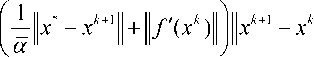
0 <  f ( x^k ) - f ( x *) < / -1 ( x* - x^{k + 1} ) - f '( x^k ), x^{k + 1} - x^k ) <

Since M ( x ⁰ ) is bounded, then

||x* - x^{k + 1}11 <  sup || x - y || = K < +ro x , y e M ( x ⁰)

loT'Cxk )| - I |f( xk) - f'(x °) + f( xk )| < | If 4 xk) - f'(x 0)||+1f'(x 0)|| < L\\x - x °|| + ||f'(x °)|| < L - K + N, where N-||f'(x 0)||, x e M (x °). Then

0 < f ( x k ) - f ( x *) <| K + L - K + N ||| x^{k + 1} - x^k |I. V a            J"

Taking into account (3.8) that k™l x+1 -xkl I-0

we have lim f (xk) - f (x*)

k ^m which proves the assertion.

Numerical Experiments

The proposed algorithms for quadratic maximization and minimization problems have been tested on the following type problems. The algorithms are coded in Matlab. Dimensions of the problems were ranged from 200 up to 5000. Computational time, and global solutions are given in the following tables.

Problem 1.

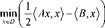
max x e D

(( Ax, x ) + B, x ^)

subject to where

D - { - ( n - i + 1 ) <  x i <  n + 0.5 i, i - 1,2,..., n }

( n n - 1

n - 1 n

V 1      2

n J

B - (1,1,...,1)

Problem 2.

subject to

Problem 3.

n max ^ (n -1 - 0.1 - i)xi2

i - 1

D - { x e R n I - 1 - i <  x i <  1 + 5 i ,   i - 1,2,..., n }

subject to

where

D = { 10 < x_t <  30, i = 1,2,..., n }

	^ n n - 1 .	. 1 >
	n - 1 n .	.. 2
A =			, b = (1,1,...,1)
	. 1        2 L	- n ;

Problem 4.

n mm« S( x -1)2

l = 1

subject to

D = { x e Rⁿ I i + 1 <  x <  i + 10, i = 1,2,..., n }

Table

proble m	n	Initial value	Global value	Computing time (sec)
1	200	2.66690000000000e+006	335.337841669956e+009	4.166710
1	500	41.6672500000000e+006	32.7084036979206e+012	29.082187
1	1000	333.334500000000e+006	1.04625056270796e+015	202.615012
1	2000	2.66666900000000e+009	33.4733378341612e+015	1579.706486
1	5000	41.6666725000000e+009	3.26848965365074e+018	22248.485127
2	200	37.7900000000000e+003	12.3936575899980e+009	4.766626
2	500	236.975000000000e+003	482.716617724994e+009	30.115697
2	1000	948.950000000000e+003	7.71590814447147e+012	196.977634
2	2000	3.79790000000000e+006	123.393965944640e+012	1786.474928
2	5000	23.7447500000000e+006	3.5660855482763485e+18	27342.423215
3	200	600.004500000000e+006	266.668000000000e+006	9.625021
3	500	9.37501125000000e+009	4.16667000000000e+009	69.149144
3	1000	75.0000225000000e+009	33.3333400000000e+009	408.735783
3	2000	600.000045000000e+009	266.666680000000e+009	3035.512940
3	5000	937.500011250000e+012	416.6666800000000e+12	21432.421674
4	200	500	200.00	9.227003
4	500	12500	500.00	56.679240
4	1000	25000	1000.00	365.62471
4	2000	50000	2000.00	2904.275652
4	5000	125000	5000.00	22134.532145

Conclusion

To provide a unified view, we considered the quadratic programming problem consisting of convex quadratic maximization and convex quadratic minimization. Based on global optimizality conditions by Strekalovsky [11, 12] and classical local optimality conditions [1, 7], we proposed some algorithms for solving the above problem. Under appropriate conditions we have shown that the proposed algorithms converges to a global solution in a finite number of steps. The Algorithm MAX generates a sequence of local maximizers and and uses linear programming at each iteration which makes algorithm easy to implement numerically.