Machine Learning-based Approaches in Error Detection and Score Prediction for Small Arm Firing Systems in the Military Domain

Published Online on April 8, 2024 by MECS Press

The traditional approach to military shooting evaluation involves firing shots from different positions and phases, assessing accuracy based on a 10-inch diameter target. The process relies on manual measurement using a ruler, and data is subsequently entered into a database. This method is time-consuming, prone to human error, and lacks the efficiency required for modern military operations. To address these shortcomings, the military must consider the integration of an automated firing assessment system. The current military evaluation of shooting performance relies on a senior fully manual process. Shots are fired from various locations and positions during different phases to assess whether they hit the target within a 10-inch diameter. Success results in credit, while failure is termed a washout. Measurement of the 10-inch diameter is performed using a ruler. Subsequently, the observer approaches the target, examines the impact using the ruler, and manually enters the data into a database or records. This approach is timeconsuming, inefficient, and labor- intensive. Consequently, there is a need to reevaluate the existing shooting scoring system and implement an automated firing assessment system for improved speed and efficiency. To sum up, in order to stay competitive and make the most use of training resources, military shooting evaluation must be updated. Increasing speed, accuracy, and efficiency through the use of an automated shooting evaluation system will ultimately improve armed forces’ overall preparedness and efficacy. To adapt to the changing needs of modern warfare, military institutions must embrace technological breakthroughs.

Assessing an individual’s firing performance in the military is inherently challenging due to the intangible nature of shooting skills and the lack of a precise criterion for measurement. With many military personnel undergoing firing exercises only sporadically, and some having limited opportunities, perhaps once or twice a year, there is a critical need for a comprehensive evaluation system. Such a system should not only provide accurate judgments of firing performance but also ensure easy accessibility, catering to the diverse training schedules of military personnel. An accessible firing evaluation system becomes pivotal in enhancing the shooting skills and overall performance of individuals, ensuring that they are adequately prepared for the demands of their roles.

In addition to accuracy and accessibility, the development of a robust storage system for maintaining records is imperative. Military organizations must have the capability to track and analyze historical firing data to identify trends, strengths, and areas for improvement. This historical perspective can inform targeted training programs and facilitate a more strategic approach to skill development. Moreover, a forward-looking firing assessment system that can predict future performances for individual firers would be transformative. By leveraging predictive analytics and machine learning, the system can offer insights into potential areas of improvement, allowing military personnel to proactively address skill gaps and optimize training regimens. In essence, a comprehensive and predictive firing assessment system holds the promise of making a transformative impact in the military, contributing significantly to the ongoing improvement of individual and collective firing skills.

Leveraging machine learning (ML) for the identification of bullet holes in the aftermath of military firing exercises represents a cutting-edge advancement with profound implications for post-firing assessments. The work by [1] underscores the potential of ML algorithms to enhance precision and efficiency in detecting and analyzing bullet holes. By automating the identification process, these algorithms alleviate the burden of manual inspection, enabling real-time assessment and expediting the overall evaluation procedure. The practical application of ML in bullet hole detection, as demonstrated by [2], not only streamlines the evaluation process but also offers the military a data-driven approach to refine training protocols and enhance decision-making processes. This technological integration holds the promise of elevating the overall readiness and effectiveness of military operations by providing more accurate and timely insights into shooting performance.

Moreover, ML-based bullet hole detection systems extend their utility beyond assessment, contributing to firearm safety and operational efficiency. As highlighted by [3], these systems can identify anomalies and malfunctions in firearms, enabling proactive maintenance measures to sustain optimal firearm performance. This preventive aspect not only ensures the safety of military personnel but also mitigates the risk of potential incidents related to weapon malfunction. The development and integration of ML-driven technologies in the realm of military firing exercises thus emerge as a transformative asset, fostering improved safety protocols, operational efficiency, and overall effectiveness in military training and operations.

While there is a notable absence of research specifically addressing the automation of error pattern recognition systems and performance predictions in the military domain, several studies in other fields have explored the application of machine learning algorithms for similar purposes. Notably, the implementation of algorithms such as Random Forest and AdaBoost has been investigated in diverse contexts to recognize patterns and forecast performance outcomes.

Based on our military domain, we proposed two algorithms in this paper.

• •    Random Forest classifier to recognize error patterns based on the spreading of bullets on target paper because of its ability to improve the accuracy of predictions by combining the results of multiple decision trees. An ensemble classification strategy devised by Breiman has shown exceptional performance in terms of prediction error on a collection of benchmark datasets. To the best of our knowledge, this is the inaugural effort where a random forest classifier has been successfully applied to a real-time bullet hole dataset within a genuine scenario.

• •    Adaboost classifier to predict the score and performance of soldiers based on selective constraints because of its ability to improve the accuracy of predictions by iteratively adjusting the weights of incorrectly classified instances. To the best of our knowledge, this is the inaugural effort where an Adaboost classifier has been

2.    Military Firing System and Related Work 2.1.    Military Firing System

successfully applied for the score performance.

The paper will initially present a concise literature review. Workflows will be used to illustrate the methodology of this research in depth. The discussion will conclude with comparative results and final remarks.

The current methodology employed by the military for recognizing patterns of error in shooting targets involves a fully manual approach, as depicted in Figure 1. This labor-intensive process relies on active human participation to analyze firing images, visually interpret bullet spread patterns on target paper (as illustrated in Figure 2), and classify errors into specific types such as Long Horizontal Error (X1), Long Vertical Error (X2), Bi-Focal Error (X3), Scattered Error (X4), or the absence of an error (X5). Subsequently, shooters are provided with correction guides based on identified error patterns. The existing system is time-consuming and demands significant human effort, making it less than ideal for modern military training scenarios. To enhance efficiency and effectiveness, there is a compelling need for an automated error pattern recognition system that can swiftly analyze firing images, classify errors, and provide corrective guidance without the same level of manual intervention.

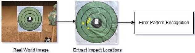
Fig.1. Error pattern recognition in military domain

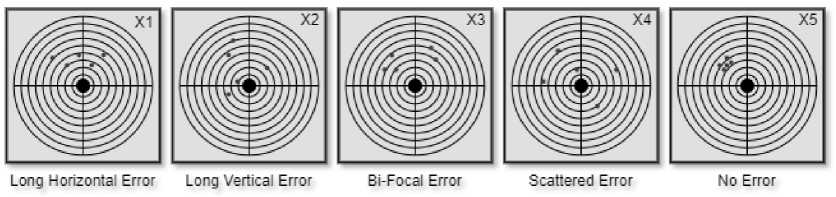
Fig.2. Various error patterns based on spreading of bullets on target paper

In a parallel context, the military’s score and performance prediction system also currently rely on manual strategies, considering factors such as previous shooting results and other contextual circumstances. However, these approaches are neither quick nor efficient, often demanding substantial labor. There is a clear opportunity to revolutionize this aspect by developing an automated system capable of recognizing error patterns and predicting the future performance of a shooter. Such a system, integrating machine learning and pattern recognition algorithms, could provide timely insights, streamline the correction process, and contribute to more effective training regimens, ultimately enhancing the overall readiness of military personnel. Therefore, a paradigm shifts towards an automated error pattern recognition system coupled with score prediction is crucial to bring about advancements in the evaluation and enhancement of shooting skills in the military domain.

• 2.2.    Related Work

• A.    Bullet Hole Using Image Processing

In a research endeavor conducted by [4], a comprehensive automatic scoring system for live shooting sessions is delineated. This innovative system leverages advanced image processing techniques and incorporates a camera strategically positioned in front of the shooting target frame. The methodology integrates various image processing algorithms, including target ring identification, perspective transformation, image subtraction, and morphological image processing. The operational sequence encompasses the recording of individual shots on 10 target sheets, each featuring 10 bullet hole photos meticulously captured through circular stickers. This inventive approach, grounded in computer vision for target detection, is specifically acknowledged for its cost-effectiveness compared to conventional shooting target scanners or optical evaluation systems.

The automatic shooting scoring architecture consists of four main processes: image perspective transformation, scoring circle detection, bullet hole detection, and scoring mechanism. However, the study highlights challenges related to the sensitivity of the image subtraction method, leading to potential inaccuracies due to changes in external conditions, such as lighting variations. The image subtraction process, while effective in detecting bullet holes, can introduce noise, impacting the precision of the scoring process.

In a separate study by [5], researchers employed image processing techniques for bullet detection, specifically focusing on eliminating the impact of gunshot holes on the background. This method, designed for indoor shooting scenarios, achieved a 100% accuracy rate in bullet detection. The researchers utilized background subtraction and Euclidean Distance Methods to build an automatic shooting scoring system. The background subtraction technique detected previous shot holes, while the Euclidean Distance method measured the distance between holes and the center point, enabling automatic score calculation.

The image processing steps involved in this research include transforming the gunshot image, cropping the shot, detecting circle assessments, detecting shot marks, and an automatic assessment process. The study notes that the intensity of light can influence the detection results of shot holes, with very dark conditions reducing accuracy. However, under normal lighting conditions (measured in the range of 80 lux to 120 lux), the system demonstrated proper detection and achieved a 100 percent accuracy rate.

In summary, these studies showcase the application of image-processing techniques for automatic scoring systems in live shooting sessions. While effective, challenges related to sensitivity to external conditions and lighting variations highlight the need for robust algorithms and system adjustments to ensure precision and reliability in scoring processes.

• B.    Bullet Hole Using Machine Learning

In this section, we will discuss the machine-learning approaches used in bullet holes using machine learning. Several recent literature bases on machine learning have addressed this issue of bullet holes [4,5,6-9].

In the military context, small arms shooting practices demand precise analysis of bullet groups to assess weapon precision and shooter accuracy. Traditional manual or semi-automatic methods using image processing lack adaptability to environmental conditions. This paper introduces a novel approach employing deep learning techniques, specifically Mask R-CNN for target segmentation and ResNet-50 for bullet hole detection, achieving significant success in real-time shooting system automation. Experimental results demonstrate an average precision of 0.87 for target segmentation with Mask R-CNN and 0.80 for bullet hole detection with ResNet-50 on real-time datasets.

In [7] authors aim to present a study on the automatic classification of bloodstain patterns caused by gunshot and blunt impact at various distances. The study employs machine learning algorithms to analyze and classify bloodstain patterns based on their morphological and dimensional features. A set of features with possible relevance to classification is designed and the random forests method is used to rank the most useful features and perform classification. However, this paper doesn’t discuss comparative studies on machine learning algorithms.

In [8] Aman Sahu, Devang Kaushik, and A. Meena Priyadharsini developed a machine learning model to predict the outcome of cricket, based on individual performance, team performance, and environmental factors. These improved models can help decision-makers during cricket games. Team selection can be aided by improved models during cricket games to test team strengths against other and environmental factors. The availability of different formats and automatic machines for learning has made it important to use machine learning in this sport. The study implied a Random Forest classifier and Adaboost classifier to predict the outcomes and the pre-processing of the dataset involved the use of a label encoder.

In [6, 9], the paper describes a machine learning system for traffic flow management and control, combining Random Forests and Adaboost algorithms, which perform well on real data and can estimate and predict congestion. Traffic Delays can reduce the speed, reliability, and cost-effectiveness of the transportation system, and it is important to predict and minimize them. The use of Adaboost with Random Forest as a weak learner enables the creation of an accurate model for traffic flow prediction by considering a variety of factors such as traffic patterns, road conditions, and weather. This study proposed a hybrid Adaboost-Random Forest Algorithm for traffic congestion prediction, promising results on simulations and real data.

In [10] the author addresses the crucial role of firing and scoring in military operations, emphasizing the need for automated target scoring to reduce human error. By incorporating image processing techniques, including structural similarity indexing algorithms, the study successfully detects bullet holes in real-time military scenarios. The proposed system shows promising results in achieving automatic calculation of target scores, presenting a valuable contribution to enhancing efficiency in military evaluations.

• C.    Bullet Hole Using in Military Domain

• 2.3.    Research Gap

3.    Methodology

Automated bullet scoring plays a pivotal role in military operations by leveraging image processing techniques, particularly structural similarity indexing algorithms, to detect and evaluate bullet holes on targets. The current partially automated evaluation system necessitates manual intervention, contributing to time inefficiencies and potential human errors. This paper focuses on the design and development of a fully automatic scoring process, showcasing promising results in real-time military scenarios. By minimizing the need for manual input, this system enhances the accuracy and efficiency of target scoring, ultimately bolstering the effectiveness of military evaluations and decision-making processes [11-16].

As mentioned earlier, no research has been conducted in the military domain to recognize error patterns that improve performance in shooting targets. Different machine learning models have been created to predict outcomes and performance in other domains except the military.

We divided the whole methodology part into two modules:

• •    Module 1: Error Pattern Recognition

• •    Module 2: Score and Performance Prediction

• 3.1.    Module 1: Error Pattern Recognition

Error patterns play a crucial role in enhancing performance in shooting targets by providing valuable insights into areas for improvement. Recognizing and analyzing error patterns allows shooters to identify systematic mistakes, refine their techniques, and adjust their approach to achieve greater accuracy. Whether it involves addressing long horizontal errors, long vertical errors, bi-focal errors, or scattered errors, understanding these patterns enables shooters to implement targeted corrections and refine their skills. By leveraging error patterns as learning opportunities, individuals can develop a more precise and consistent shooting proficiency, ultimately contributing to improved performance in hitting targets within specified parameters.

• A.    Data Collection

Initially, each entry of the data set is formed with the normalized coordinates of five bullet holes shown in Table 1 that includes the coordinates of five points in a normalized graph. The graph from which the points are synthesized is shown in fig 3.

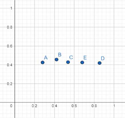
Fig.3. Synthesize normalized coordinates from graph

Table 1. Example of initial dataset for error pattern recognition

#	Point A	Point B	Point C	Point D	Point E	Error Classification
1	0.280,0.424	0.421,0.455	0.536,0.427	0.854,0.418	0.680,0.424	X1
2	0.525,0.224	0.130,0.530	0.280,0.186	0.224,0.616	0.267,0.873	X2
3	0.587,0.249	0.672,0.058	0.875,0.254	0.654,0.597	0.783,0.910	X2
4	0.314,0.302	0.3144,0.109	0.896,0.355	0.379,0.254	0.8874,0.277	X1
5	0.656,0.910	0.494,0.687	0.778,0.498	0.454,0.242	0.623,0.100	X2
.	.	.	.	.	.	.

• B.    Pre-processing

A ’scipy.spatial.distance.pdist’ function is then applied to five coordinates of the data set. The ’scipy.spatial.distance.pdist’ function calculates the pairwise distances between five 2-dimensional coordinates using the Euclidean distance metric, which is the default distance metric. The Euclidean distance between two points (x1, y1) and (x2, y2) is calculated as the square root of the sum of the squared differences of the coordinates which is formulated below.

d = ^(xl - x2)2 + (yl - y2)2)                              (1)

The ’pdist’ function calculates the Euclidean distances betwen each unique pair of points and returns the distances in a 1-dimensional array.

Table 2. Example of train/test dataset for error pattern recognition

#	Point A	Point B	Point C	Point D	Point E	Error Classification
1	1.373	0.958	0.836	1.502	0.978	X1
2	1.940	1.371	1.743	1.315	2.017	X2
3	1.542	1.888	1.641	1.641	2.550	X2
4	1.429	1.5802	1.820	1.274	1.757	X1
5	2.213	1.664	1.610	1.779	2.059	X2
.	.	.	.	.	.	.

• C.    Random Forest Classifier in Error Pattern Recognition

Random Forest is an ensemble learning method that makes predictions using several decision trees. It operates by training numerous decision trees on distinct data sub-samples and integrating their predictions via a voting procedure. The Random Forest method works in three steps:

Bootstrapping: Bootstrapping generates multiple samples from the original training data. A bootstrap sample is a random sampling of the data with replacement, which means that certain data points may be repeated while others are omitted. The Random Forest approach captures the data variability and generates a more robust model by creating many bootstrapped samples. It can be described in mathematical terms as:

Xi = {x1, x2, ..., xn}                                                   (2)

where xj ∈ X and j = 1, 2, ...n and multiple bootstrapped samples can be generated as X1, X2, ..., Xm

Training Decision Trees: The second stage involves training decision trees on each bootstrap sample. A decision tree is a tree-like structure that represents the links between data characteristics and class labels. Each node in the tree represents a data attribute, while the edges between nodes reflect the connections between attributes. The objective is to discover a model capable of properly predicting the class label of fresh data items based on their attributes. The quality of the splits at each node is defined by a measure of impurity, such as information gain or Gini impurity, which measures the degree to which the data is segregated depending on the selected characteristic. [3]. Training a decision tree works in four steps:

• •    Select a feature and threshold for splitting the data.

• •    Split the data into subsets based on the feature and threshold.

• •    Repeat the process for each subset until a stopping criterion is reached.

• •    The final output is a tree where each internal node represents a split and each leaf node represents a class prediction.

Voting: The final prediction for a new data point is made by integrating the forecasts of all decision trees in the forest. Each decision tree in the forest produces a forecast for its class label when presented with a new data point. The algorithm counts the number of decision trees that correctly predict each class label for each class label. The ultimate forecast is the class label with the highest number of votes [9].

The Random Forest technique reduces overfitting and improves the accuracy of predictions by combining the predictions of several decision trees trained on unique bootstrapped samples of the data. In addition, by training each decision tree on a different sample of data, the Random Forest technique is better able to represent the richness and diversity of the data. Figure 4 shows Train Accuracy of 1.0 and Validation Accuracy of 0.9682539682539683 for the classifier.

Mathematical Explanation of Random Forest classifier

Random Forest(D, T, m) = 1 E t=i Decision Tree(D _t , m)                       (3)

where:

• •    D is the training dataset with N samples and P features.

• •    T is the number of trees in the forest.

• •    m is the number of randomly selected features to consider for each split in the decision tree.

• •    Dt is a random subset of the training data, obtained by bootstrapping N samples from the original data with

replacement.

• •    Decision Tree (Dt, m) is a decision tree grown on the bootstrapped data Dt using only m randomly selected features at each split.

The algorithm proceeds as follows:

Algorithm 1: Solar radiation forecasting using Deep Learning Techniques

Step 1: For each tree in the forest, t = 1, ..., T:

Step 2: Randomly select N samples from the original data with replacement to create a bootstrapped dataset Dt

Step 3: Build a decision tree on Dt using only m randomly selected features at each split.

Step 4: Return the average of the predictions from all the trees in the forest as the final prediction.

Training the model: Fig 5 helps us to understand how the training and testing loss changes as the number of estimators in the random forest classifier is increased. As the number of estimators increases, the training loss decreases, meaning that the model is better able to fit the training data. The ideal number of estimators is the one that gives the best balance between over-fitting and under-fitting. In the graph, it is seen that the testing loss decreases until a certain point and then begins to increase again. The point at which the testing loss begins to increase is often used as a measure of the optimal number of estimators.

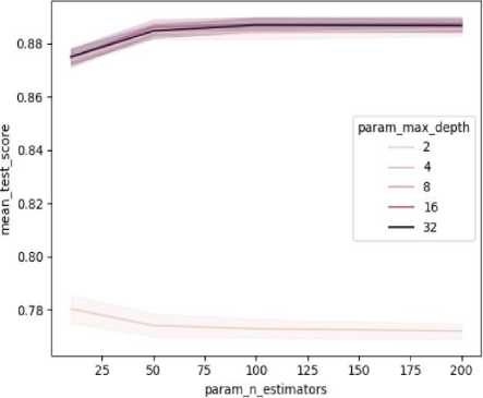
Fig.4. Hyperparameter tuning

Table 3. Hyperparameter random forest

Param_n_estimators	Param_max_depth	Param_criterion	Mean_test_score	Std_test_score
100	10	gini	0.897491039	0.088888889
20	8	gini	0.897388633	0.070340221
50	8	gini	0.897388633	0.070340221
20	10	gini	0.89421403	0.077215051
30	10	gini	0.891141833	0.094096996
100	8	gini	0.89109063	0.08623848
10	8	gini	0.884639017	0.098672528
30	8	gini	0.884639017	0.086896743
50	10	gini	0.884639017	0.08259925
10	10	gini	0.878187404	0.090587613

Hyper parameter tuning of Random Forest classifier: Fig 4 shows the hyperparameter tuning for the Random Forest Classifier. It’s seen that for n estimators value of 100, max depth of 10, and parameter criterion set to ’gini’ the model shows the highest test score. Using 100 estimators means that 100 decision trees are trained and used to make predictions, and this led to improved performance compared to using a smaller number of trees because it provides a more diverse set of predictions and reduces the variance in the model. The choice of the ’gini’ impurity criterion results in a more homogeneous prediction, which helps to increase the accuracy of the random forest.

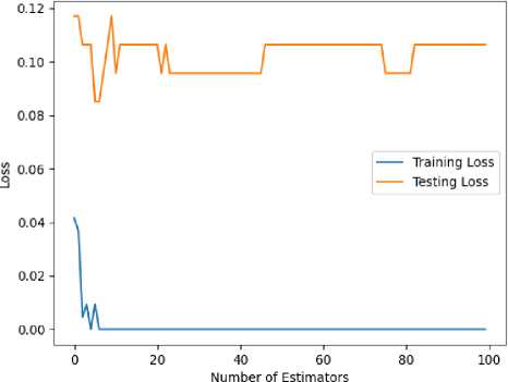
Fig.5. Train-test loss function for random forest

• 3.2.    Module 2: Score and Performance Prediction

• 3.3.    Dataset Collection and Processing

• 3.4.    Adaboost Algorithm

Score and performance prediction for soldiers during shooting in the military domain is a critical aspect of enhancing training effectiveness and operational readiness. Leveraging machine learning algorithms can provide valuable insights into individual and collective shooting capabilities, allowing for targeted improvements and informed decision-making. By analyzing historical shooting data, including factors such as accuracy, consistency, and reaction time, predictive models can be developed to forecast a soldier’s future performance. These models may consider variables like weapon proficiency, environmental conditions, and stress levels to provide a holistic assessment. The implementation of such predictive analytics not only aids in identifying areas for improvement but also assists in optimizing training programs, resource allocation, and overall military preparedness. Integrating real-time feedback mechanisms can further enhance the adaptability of training regimens, ensuring that soldiers are well-prepared for diverse and challenging scenarios in the field. Over- all, score and performance prediction in the military domain contribute significantly to the continuous improvement of shooting skills, fostering a more effective and responsive military force.

The second module’s data set consists primarily of 16 features provided over a one-year period, which include Army No., Rank, Name, Service Length, Wind (Force), Wind (Direction), Temperature, Weather, Light, Zeroing of Weapon, Type of Ammo, Type of Range, Type of Fire, Grouping, Hit Fire and ETS. The data pre-processing operations consisted Creation of a new variable, Label Encoding, and Normalization. From the variable importance graph shown in 6 for the train-test dataset, we can see that the service length metric has the highest importance because as the soldier’s age increases, his or her experience also increases.

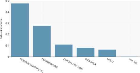
Fig.6. Variable importance

AdaBoost is a meta-algorithm for statistical classification that uses ensemble learning to enhance performance by combining the outputs of multiple “weak learners.” It modifies subsequent weak learners to prioritize misclassified samples, resulting in a final model that converges to a strong learner. AdaBoost is commonly used with decision trees as the weak learners and is often cited as the most effective classifier out-of-the-box. It feeds information on the difficulty of classifying each sample into the decision tree learning process, leading to later trees focusing on harder samples. Fig 7 is a depiction of the overall structure of the Adaboost classifier.

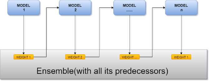
Fig.7. Architecture of adaboost classifier

Mathematical Explanation of Adaboost Classifier

AdaBoost can be mathematically defined as follows:

Adaboost(D,T) = X t=i a_th_t(x)

where:

• - D = {(x1, y1), ..., (xN , yN )} is the training dataset with N samples and P features - T is the number of weak classifiers used in the boosting process - ht(x) is the tth weak classifier - αt is the weight assigned to the tth weak classifier

The Adaboost algorithm is an iterative process that assigns weights to the training samples and trains a series of weak classifiers. The steps involved in the Adaboost algorithm are as follows:

Algorithm 2: Random Forest Classifier in error pattern recognition Step 1: Initialize the weights wi = 1/N

Step 2: For each iteration t = 1, ..., T: for each sample in the training data

Step 3: Train a weak classifier ht(x) on the weighted training data Step 4: Compute the weighted error rate of the weak classifier:

N tt

= ^w_i[y_i * h t (Xi')] i=i

Step 5: Compute the weight αt for the weak classifier:

^a t = 1 log

1-Et

^E t

Step 6: Update the weights of the training samples:

The weights are re-normalized so that they sum up to 1.

Step 7: Return the final prediction as a weighted sum of the predictions from all the weak classifiers:

T

f(x) = Sign I )     a t h _t (x)

Hyper parameters of Adaboost Classifier: AdaBoost has several hyperparameters that can be adjusted to control the behavior of the model which is shown in table 4. Here, n estimators is the number of weak models (decision stumps) that will be trained in the ensemble. The learning rate determines how much each weak model contributes to the final prediction. A slower learning rate means that each weak model adds less to the final prediction. This makes convergence slower, but the model is more reliable.

Table 4. Hyper parameter tuning of Adaboost classifier

n_estimetor	Learning Rate	Accuracy	Precision	Recall	F1 Score
20	.5	.5952380	.3715728	.5952380	.4575337
30	.5	.6904761	.5648970	.6904761	.6198776
30	1	.5654761	.3939707	.5952380	.4627439
70	.5	.5833333	.3894039	.5952380	.4661218
100	.5	.5714285	.3937012	.5952380	.4651027
100	1	.5178571	.4250927	.5178571	.4633306
200	.5	.4904761	.4277883	.4904761	.4550350
200	1	.4900021	4280125	.4904761	.4752369

Adaboost Classifier in Score Prediction

The AdaBoost (Adaptive Boosting) algorithm is a powerful ensemble learning technique designed for binary classification tasks. The initialization step sets equal weights for all training data points. Subsequently, a series of weak models, typically decision stumps, are trained on the weighted training data in an iterative manner. During each iteration, the decision stump makes predictions, and the weights of misclassified samples are increased. The weights of the training samples are then updated based on the accuracy of the current weak model. This process is repeated until a predefined number of weak models are trained or a satisfactory level of accuracy is achieved. The final prediction is made by combining the predictions of all weak models through a weighted majority vote, where the weights are determined by the accuracy of each weak model. Finally, the performance of the ensemble model is evaluated using standard metrics such as accuracy, precision, recall, and F1-score to assess its effectiveness in capturing the underlying patterns in the data and making accurate predictions.

Algorithm 3: Adaboost Classifier in score Prediction

Step 1: Initialization: The weights of all training data points are set to be equal.

Step 2: Training: A weak model (decision stump) is trained on the weighted training data. The decision stump makes predictions on the training data and the weights of the misclassified samples are increased.

Step 3: Weight update: The weights of the samples are updated based on the accuracy of the current weak model.

Step 4: Repeat: Steps 2 and 3 are repeated until the desired number of weak models are trained or a satisfactory level of accuracy is reached.

Step 5: Prediction: The final prediction is made by combining the predictions of all weak models using a weighted majority vote, where the weights are determined by the accuracy of each weak model.

Step 6: Evaluation: The performance of the final model is evaluated using appropriate evaluation metrics such as accu- racy, precision, recall, F1-score, etc.

4.    Results

In this experimental section, a comprehensive investigation was conducted, encompassing a diverse range of machine- learning algorithms. Numerous experiments were executed to assess the performance and efficacy of these algorithms in addressing the research objectives. The experimentation involved rigorous testing and evaluation, considering factors such as algorithmic accuracy, computational efficiency, and the ability to handle diverse datasets. The results obtained from these experiments are pivotal in shedding light on the comparative strengths and weaknesses of the various machine- learning approaches employed.

• 4.1.    Evaluation Metrics

• 4.2.    Module 1: Error Pattern Recognition

Several performance metrics are commonly employed to evaluate the effectiveness of classifiers based on the information contained in the confusion matrix. The following measures are frequently utilized:

Accuracy: This metric provides an overall assessment of the classifier’s correctness by calculating the proportion of correctly classified instances. While it offers a quick overview of performance, accuracy can be misleading in imbalanced datasets where one class significantly outweighs the others. It is expressed as (TP + TN) / (TP + TN + FP + FN), representing the proportion of accurately predicted cases.

Precision: Precision evaluates the classifier’s capability to correctly identify positive instances without mislabeling negative examples as positive. It is calculated as the fraction of true positive cases relative to the total number of predicted positive examples, expressed as TP / (TP + FP). High precision indicates a low false positive rate, which is crucial in applications where incorrect positive predictions can be costly or risky.

Recall: This metric assesses the classifier’s ability to identify all positive instances and is the ratio of true positive cases to all actual positive instances, given by TP / (TP + FN). High recall signifies a low false negative rate, which is vital in applications where erroneous negative predictions can be detrimental.

F1 Score: The F1 score represents the harmonic mean of precision and recall, offering a balanced measure between the two. It assigns equal weight to accuracy and recall, and a high F1 score indicates a classifier with both good precision and recall. Mathematically, it is computed as 2 * (Precision * Recall) / (Precision + Recall).

According to the Standard Operating Procedure of the Armed Forces, the error is categorized into four categories based on the pattern of bullet spread. Figure 2 shows Long Horizontal Error as X1, Long Vertical Error as X2, Bi-Focal Error as X3, Scattered Error as X4, and another condition where no error is recognized as X5.

• A.    Random Forest

A visual representation of the performance of the Random Forest classifier is shown in figure 8 as confusion matrix. In this case, with five labels (X1, X2, X3, X4, and X5), the matrix would be a 5x5 grid where the rows represent the true class of each instance, and the columns represent the predicted class. In this scenario, the values along the diagonal of the matrix are high and the off-diagonal values are absent, indicating that the classifier is accurately predicting the true class of each instance.

• B.    Support Vector Machine

A visual representation of the performance of the Support Vector Machine (SVM) classifier is shown in figure 9 as a confusion matrix. In this case, with five labels (X1, X2, X3, X4, and X5), the matrix would be a 5x5 grid where the rows represent the true class of each instance, and the columns represent the predicted class. In this scenario, the values along the diagonal of the matrix are high, and the off-diagonal values are present, indicating that some values were misclassified by the SVM classifier.

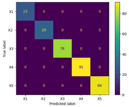
Fig.8. Confusion matrix of random forest

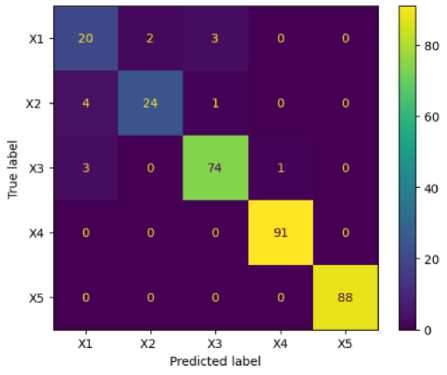
Fig.9. Confusion matrix of SVM

• C.    K-Nearest Neighbors

A visual representation of the performance of the K-Nearest Neighbors (KNN) classifier is shown in figure 10 confusion matrix. In this case, with five labels (X1, X2, X3, X4, and X5), the matrix would be a 5x5 grid where the rows represent the true class of each instance, and the columns represent the predicted class. In this scenario, the values along the diagonal of the matrix are high and the off-diagonal values are present, indicating that some values were misclassified by the K-Nearest Neighbors (KNN) classifier.

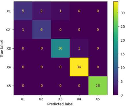
Fig.10. Confusion matrix of K-NN

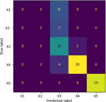
Fig.11. Confusion matrix of decision tree

• D.    Decision Tree

A visual representation of the performance of the decision tree classifier is shown in figure 11 as confusion matrix. In this case, with five labels (X1, X2, X3, X4, and X5), the matrix would be a 5x5 grid where the rows represent the true class of each instance, and the columns represent the predicted class. In this scenario, the values along the diagonal of the matrix are high and the off-diagonal values are present, indicating that some values were misclassified by the decision tree classifier. It also appears that for X1 and X2 the model completely failed to predict accurately.

• E.    Neural Network

• 4.3.    Module 2: Score and Performance Prediction

Table 5 represents the accuracy, precision, recall, and F1 score of the neural network algorithm where the loss function is a mean squared error (MSE) and the metric used to evaluate the model is also MSE, the optimizer is set to Adam with a learning rate of 0.01, and the batch size is 256 with 300 epochs.

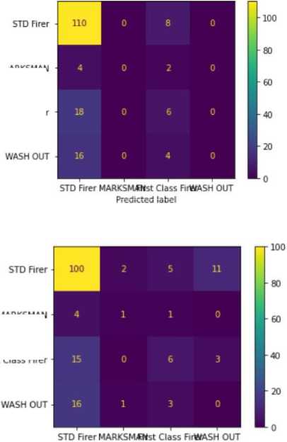
• A.    Adaboost

In this particular illustration 12, the Adaboost classifier made an accurate prediction of 110 STD Firers and 6 First Class Firers. These are the values that are located along the diagonal of the matrix. On the contrary, the classifier incorrectly identified 8 STD Firers as First Class Firers, 4 Marksman as STD Firers, 2 Marksman as First Class Firers,

18 First Class Firers as STD Firers, 16 Washouts as STD Firers and 4 Washouts as First Class Firers; these values may be found in the cells that are located off to the side of the diagonal.

£

£

First Class Finer

Fig.12. Confusion matrix of Adaboost

Predicted label

MARKSMAN

MARKSMAN

First Class Firer

Fig.13. Confusion matrix of decision tree

• B.    Decision Tree

In the decision tree, the classifier correctly predicted that there would be 100 STD Firers, 1 Marksman, and 6 First Class Firers. In contrast, the classifier made some erroneous judgments, mislabeling 2 STD Firers as Marksman, 5 STD Firers as First Class Firers, 11 STD Firers as Washouts, 4 Marksman as STD Firers, 1 Marksman as First Class Firers, 15 First Class Firers as STD Firers, 3 First Class Firers as Washouts, sixteen Washouts as STD Firers, 1 Washout as Marksman and 3 Washouts as First Class Firers as we see in 13. The classifier failed to detect any Washouts.

STD FIRER

MARKSMAN

First Class FIRER

WASH OUT

Predicted label

Fig.14. Confusion matrix of random forest

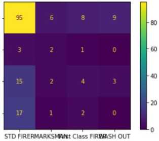
• C.    Random Forest Classifier

The classifier accurately predicted that there would be 95 STD Firers, 2 Marksman, and 4 First Class Firers based on the Random Forest Algorithm. In contrast, the classifier made some incorrect assessments, mislabeling 6,8,9 STD Firers as Marksman, First Class Firers, and Marksman respectively, 3 Marksman as STD Firers, 1 Marksman as FirstClass Firers, 15 First Class Firers as STD Firers, 2 First Class Firers as Marksman, 3 First Class Firers as Washouts, 17 Washouts as STD Firers, 1 Washout as Marksman, 2 Washouts as First Class Firers depicted in 14. The classifier was unable to spot any Washouts.

STD Firer

_ MARKSMAN jo ф

First Class Firer

WASH OUT

107	0	0	0
12	0	0	0
24	0	0	0
25	0	0	0

STD Firer MARKSMANst Class FirWASH OUT Predicted label

Fig.15. Confusion matrix of SVM

• D.    SVM Classifier

The classifier accurately predicted that there would be 107 STD Firers. But wrongly predicted 12 Marksman, 24 First Class Firers, and 25 Washouts as STD Firers as depicted in 15. The classifier predicts every entry as STD Firers.

STD Firer

MARKSMAN

First Class Firer

WASH OUT

	0	1	0
10	0	2	0
21	0	3	0
25	0	0	0

STD Firer MARKSMJfNst Class FirWASH OUT Predicted label

Fig.16. Confusion matrix of naive bayes classifier

• E.    Naive Bayes Classifier

• 4.4.    Comparative Analysis

• A.    Module 1 - Error Pattern Recognition

The comparative analysis presented in Table 5 reveals that the random forest classifier outperforms other algorithms in the context of score prediction for error pattern recognition. The superior performance of Random Forest can be attributed to its inherent strength in handling non-linear relationships between features. Its ensemble of decision trees and the aggregation of their outputs contribute to robust predictions, especially when the underlying patterns in the data are complex and intricate. In contrast, the Support Vector Machine (SVM) demonstrated competitive performance, particularly be- cause the data was separable by a linear boundary, and the training examples were limited. SVM excels in scenarios where a clear linear distinction exists between classes, making it an effective choice for certain types of datasets.

However, the neural network model’s performance lagged, primarily due to the limited amount of available training data. Neural networks, especially deep learning architectures, often require large datasets for effective training and learning of complex patterns. With a scarcity of training examples, the neural network struggled to generalize well and capture the nuances of the error patterns. This underscores the importance of considering the characteristics of the dataset and the algorithm’s suitability for the task at hand, as evidenced by the notable discrepancy in performance among the evaluated algorithms.

• B.    Module 2: Score and performance Prediction

5.    Conclusions

The analysis presented in Table 6 indicates that the AdaBoost classifier emerges as the top performer in score prediction among the considered algorithms. The notable success of AdaBoost can be attributed to its ensemble learning approach, which combines multiple weak learners, often decision stumps in this context, to form a robust and accurate overall model. The collaborative nature of AdaBoost, where each subsequent weak model focuses on the misclassified instances by its predecessors, contributes to the algorithm’s ability to adapt and improve iteratively. This results in a powerful ensemble model that excels in capturing the underlying patterns within the data.

Table 5. Aggregated result of error pattern recognition

Algorithm	Accuracy	Precision	Recall	F1 Score
Random Forest	0.96880902	0.95756571	0.95880902	0.96558131
Support Vector Machine	0.95744680	0.96247889	0.95744680	0.95995625
K-Nearest Neighbour	0.95744680	0.95889057	0.95744680	0.95816814
Decision Tree	0.90425531	0.92747545	0.90425531	0.91571820
Neural Network	0.36507936	0.37539682	0.36507936	0.37016621

On the contrary, the Naive Bayes model demonstrated suboptimal performance, emphasizing the challenge it faces in capturing intricate and complex relationships between features. Naive Bayes assumes independence between features, which might not hold in scenarios with intricate interdependencies. Consequently, when faced with the nuanced patterns within the dataset, Naive Bayes struggled to provide accurate predictions. This discrepancy in performance underscores the importance of selecting algorithms that align with the underlying characteristics of the data and the complexity of the relationships being modeled. The success of AdaBoost in this experiment showcases the efficacy of ensemble learning in enhancing predictive accuracy and robustness.

Table 6. Aggregated result of score prediction

Algorithm	Accuracy	Precision	Recall	F1 Score
Adaboost	0.69047619	0.5648970	0.6904761	0.6198776
Decision Tree	0.63095238	0.5747747	0.6309523	0.6309523
Random Forest	0.60119040	0.5578671	0.6011904	0.5758218
SVM	0.63690476	0.40564767	0.63690474	0.49562770
Naive Bayes	0.64880952	0.48816872	0.64880952	0.53051867

For this study, we proposed utilizing the Random Forest algorithm for error pattern recognition and the Adaboost algorithm for predicting shooting performance within the military domain. The study involved a comprehensive process, including data collection, modification, and pre-processing. To ensure a robust evaluation, we compared the performance of Random Forest, AdaBoost, Decision Tree, Support Vector Machine (SVM), Naive Bayes, K-Nearest Neighbor, and Neural Network algorithms. The results from both modules, error pattern recognition, and shooting performance prediction, demonstrated satisfactory outcomes. However, acknowledging the necessity for real-world validation, it is imperative to test the system in a military environment to assess its efficacy under actual operational conditions. Despite the need for further validation, the study provides promising insights, suggesting that a system employing similar algorithms could prove highly beneficial within the military domain.

In conclusion, the proposed system, leveraging Random Forest and AdaBoost algorithms, holds significant promise for improving the efficiency and accuracy of error pattern recognition and shooting performance prediction. While the study lays a solid foundation, real-world testing will be crucial to ascertain its practical utility in military applications, ensuring that the system meets the dynamic and demanding conditions of military operations.