Managing Lexical Ambiguity in the Generation of Referring Expressions

Published Online July 2013 in MECS DOI: 10.5815/ijisa.2013.08.04

Referring expressions are noun phrases (NPs) that identify particular domain entities to a hearer. The Generation of Referring Expressions (GRE) is an integral part of most Natural Language Generation (NLG) systems [1]. The GRE task can informally be stated as follows. Given an intended referent (i.e., the object to be identified) and a set of distractors (i.e., other objects that can be confused with the referent), the task is to find a description that allows a hearer to identify its referent uniquely [2]. Such a description is called a Distinguishing Description (DD), and the description building process itself is usually referred to as content determination for referring expressions. The DD is usually a logical formula or a set of properties, rather than natural language descriptions (exceptions are [3-6] which produce actual words).

One of the most widely studied GRE algorithm is Dale and Reiter’s Incremental Algorithm [7]. The algorithm aims to generate distinguishing descriptions which mimic human produced descriptions, and which can be generated as efficiently as possible. Rather than focusing on the briefest possible description (cf. Dale’s Full-Brevity Algorithm [2]), the Incremental Algorithm also generates over-specified descriptions just as speakers often do. The algorithm assumes a preference order, in which properties occur in order of their salience (or, more precisely, the order in which the algorithm will consider them).

Given an intended referent r and a set C of distractors, the Incremental Algorithm iterates through an ordered list P of properties, adding a property to the description S of r only if it is true of r and at the same time it rules out some of the distractors that have not already been ruled out. The distractors that are ruled out are removed from C . The type property (which would be realized as a head noun) is always included even if it has no discriminatory power. The algorithm terminates when a DD for r is constructed (i.e., success) or list of properties P is exhausted (i.e., failure). Later on, the DD is realized as a natural language description by a surface realiser. However, linguistic ambiguities can be introduced in the step from properties to language descriptions as shown in the following example adopted from [5].

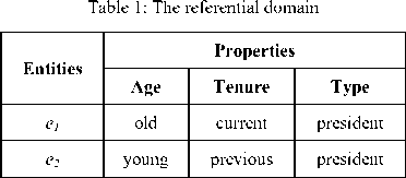
Consider the referential domain in Table 1, in which entities are charaterised as having a set of properties. (In this article, we shall represent properties as attributevalue pairs (e.g., ), and words/lexical units themselves as lowercase italics.) Also assume that the properties and are associated with the word old , that is, the word old is polysemous or lexically ambiguous. Let our task be to single out the entity e 1 from e 2 . Assume that the attribute preference is from left to right, i.e. age will be considered first, then tenure and so on.

The Incremental Algorithm will proceed as follows. The algorithm will first take the property , which is true of the intended referent (e 1 ) and also rules out a distarctor (e 2 ), and add it into the description S . At this point there are no distractors left in the distractor set, so the algorithm will add the type property (which is not already added) in the description S . The algorithm would return the distinguishing description as a logical formula: ∧ . This formula uniquely identifies the intended referent ( e₁ ) as this combination of properties does not apply to the other entities (namely, e 2 ) in the KB. The problem could arise, however, when a surface realiser would express this formula as the old president . The English NP could be interpreted as:

• (1)     ∧ , or

• (2)     ∧

Both interpretations are possible in the given domain: (1) refers to e₁ , whereas (2) refers to e₂ . Therefore, the NP is referentially ambiguous, that is, confusing as to what the intended referent of this NP is.

In this article, we examine how to deal with linguistic ambiguities which could cause referential ambiguity, focusing on lexical ambiguity.

The rest of this article is organized as follows. In Section 2, we discuss the existing approaches to deal with the lexical ambiguity in GRE. Section 3 describes our own approach followed by general discussion in Section 4. The article concludes in Section 5.

• II.    GRE and Lexical Ambiguity

• 2.1    Dealing with Lexical Ambiguity in GRE

Most GRE algorithms do not take lexical ambiguity into account because they focus only on content determination and assume that the properties accumulated by them would be realized unambiguously by words [1, 2, 8-11]. Generally, these algorithms assume a one-to-one mapping between properties and words. That is, these algorithms assume that every property can be expressed unambiguously by words in a language. However, in natural languages, a word can express more than one properties (lexical ambiguity), and conversely a property can be expressed by more than one words. When these properties have different extensions, lexical ambiguity can cause referential ambiguity (as shown in the above example).

There is very little work reported in the literature on GRE which deals with lexical issues, particularly lexical ambiguity. One work which deals with the lexical ambiguity issue in GRE is [5]. In [5], Siddharthan and Copestake proposed a greedy GRE algorithm which departs from the traditional GRE in the sense that it works at the level of words (because it takes text as its input, rather than a KB). Because they take text as input, it is important to describe how entities are characterised and constructed.

The entities are constructed from the NPs, extracted from the given text, with the head noun as type and modifiers as attributes . Like standard GRE, they also assume a closed world: the head noun and modifiers in the NP from which an entity is constructed are the only type and attributes true of the (constructed) entity. The head noun and modifiers in the NP, therefore describe the corresponding entity (constructed from the NP). It is important to mention here that Siddharthan and Copestake assume a closed world for entities: only those entities comprise the discourse, or KB in conventional GRE, which are derived from the given text.

For each adjective adj true of the intended referent, they compute a Similarity Quotient (SQ) and a Contrastive Quotient (CQ). The SQ, which exploits synonymy relationship, quantifies how similar adj is to the adjectives describing distractors, whereas the CQ, which exploits antonymy relationship, quantifies how contrastive adj is to the adjectives describing distractors. The SQ of adj is calculated by first forming sets of WordNet synonyms of adj : a set S 1 would contain WordNet synonyms of adj ; a set S 2 contain WordNet synonyms of all the adjectives in S₁; and a set S3 contain WordNet synonyms of all the adjectives in S₂. Then for each adjective describing any distractor, the SQ (of adj ) is incremented by 4 if the adjective is present in S 1 , incremented by 2 if it is present in S 2 , and by 1 if it is present in S 3 . By visiting each distractor in this manner, they keep track of the SQ of adj with respect to a particular distractor.

Similarly, the CQ of an adjective adj is computed by first forming sets of antonyms of adj : a set C₁ would contain WordNet antonyms of adj ; C₂ contain WordNet antonyms of all the adjectives in S₁ and WordNet synonyms of all the adjectives in C 1 ; C 3 contain WordNet antonyms of all the adjectives in S 2 and WordNet synonyms of all the adjectives in C 2 . Finally, the overall Discriminatory Quotient (DQ) of adj is computed as follows: DQ = CQ - SQ.

In this way, in the first step of the algorithm, they compute the DQ for each adjective true of the intended referent. These DQ values are used to construct a word preference list, in which the adjective with the highest

DQ comes first and so on. Then in a second step, they use this preference list to construct a DD (distinguishing description) in an incremental manner [7]. The pseudocode of their algorithm is given below.

Require:

An intended referent r

A set C of distractors for r, initialized to Domain – {r} A preference list L of adjectives describing r

A head noun N describing r

• 1:    Initialize the description S of r as S = ⊥

• 2:    if C = φ then

• 3:   Return N

• 4:    end if

• 5:    for each a ∈ L do

• 6:    S ← S ∧ a

% adds adjective a to S

• 7:    for each c ∈ C do

• 8:    if RulesOut(a, c) then

• 9:    C ← C \ {c}

% removes c from C

• 10:   end if

• 11:    end for

• 12:    if C = φ then

• 13:  Return S ← S ∧ N

• 14:    end if

• 15:    end for

• 16:    Return S ← S ∧ N

Siddharthan and Copestake’s Algorithm2.2    Limitations of the Existing Approach

Even though Siddharthan and Copestake’s work in GRE goes beyond content determination, it has two potential problems. First, their algorithm does not always generate distinguishing expressions, even if there exists one. This is an important limitation, because it counts against completeness of the algorithm. The fact that an adjective applies to a distractor (being synonymous with the adjectives true of the distractors) is only considered during the construction of the preference list. Once the preference list is constructed the algorithm does not exploit the similarity of the adjective true of the intended referent with any synonyms true of its distractors during the description building process. During the description building process, however, an adjective is first added to the description (cf. line 5, of the Algorithm), and then those distracters for which it has a DQ value greater than 0 are removed (cf. lines 7–9). But, an adjective having a DQ value greater than 0 with respect to a distractor does not mean that the interpretation of such an adjective would not be confused with the other adjectives describing that distractor. This is illustrated in the following example.

Consider the referential domain in Table 2. Let our task be to single out e 1 (the intended referent) from e 2

and e₃ (the distractors of the intended referent). The DQ (discriminatory quotient) values for the adjectives true of e 1 are computed; the DQ values are shown in Table 3. Therefore, the preference list would be: [ old , current , inexperienced ].

Table 2: The referential domain: the first problem

Entities	Head Noun	Attributes
e 1	president	old, current, inexperienced
e 2	president	young, previous, inexperienced
e 3	president	young, current, inexperienced

Table 3: Discriminatory quotient: the first problem

Adjective	DQ with respect to		Overall DQ
	e 2	e 3
old	2	6	8
current	4	-4	0
inexperienced	-6	-6	-12

Siddharthan and Copestake’s algorithm would take the adjective old ; add it into the description; remove e₂ and e₃ as the DQ of old is greater than 0 with respect to both e₂ and e₃ ; the DQ values are 6 and 2 respectively. (Note that the similarity of old and previous is not taken into account, while removing e 2 .) The algorithm would return a description whose realisation would be the old president .

This NP is confusing as one could interpret it as the previous president, which refers to e₂ . This means, the output of the algorithm is a non-distinguishing description. It is important to note that there exists a distinguishing description, namely, the current old president , but their approach would not produce it.

Second, at times, Siddharthan and Copestake’s algorithm produces unnecessarily long descriptions, because it adds an adjective to a description without taking into account whether or not it rules out any distractors. This limitation is illustrated in the following example.

Consider the referential domain in Table 4. Let our task be to single out e 1 from the other entities ( e 2 , e 3 and e 4 ) in the domain. The DQ values for the adjectives true of e 1 are computed as above; the DQ values are shown in Table 5.

Table 4: The referential domain: the second problem

Entities	Head Noun	Attributes
e 1	bag	small, black, striped
e 2	bag	large, white, striped
e 3	bag	large, white, striped
e 4	bag	small, black, plain

Table 5: Discriminatory quotient: the second problem

Adjective	DQ with respect to			Overall DQ
	e 2	e 3	e 4
small	4	4	-4	4
black	2	2	-4	0
striped	-4	-4	2	-6

Siddharthan and Copestake would make a preference list [ small , black , striped ]. Their algorithm would first take the adjective small ; add it into the description and remove e 2 and e 3 ; at this stage e 4 is not removed because the adjective old is non-discriminatory for e 4 . As there is still one distractor (namely, e 4 ) left, the algorithm would take the adjective black and add it into the description. The addition of the adjective black , however, is redundant as it does not remove any distractor ( black is non-discriminatory for e₄ , because DQ of black with respect to e₄ is less than 0). Finally, their algorithm would add the adjective striped into the description which successfully removes e 4 , and return the small black striped bag . This description is unnecessarily long, because it contains a superfluous adjective: the small striped bag (or the black striped bag ) could have served the purpose.

• III.    Our Treatment of Lexical Ambiguity

Our treatment of ambiguous/polysemous words is similar in spirit to that of Siddharthan and Copestake, but we use a direct extensional approach to take into account precisely how many and which distractors an ambiguous word can be regarded as true of. But the problem is how to compute the extension of an ambiguous word. The extension of a word w , written as [[ w ]], is a set of objects for which w is true. Accordingly, we compute the extension of a potentially ambiguous word by taking the union of the extensions of all its synonyms. Let the notation w:s means that w is synonym of s , and let s₁ , s₂ ,…, s_n be the synonyms of the word w , including w itself, then the extension of w is:

[[w]] = U [[s]] (Equation 1)

w : s

We suggest two changes in Siddharthan and Copestake’s algorithm. First, to remove only those distractors which do not appear in the extension of the word (being added into the description). This would solve the first problem: failure in generating distinguishing descriptions. Second, a word would be added into the description only if it removes some distractors at the present state of the task (similar in spirit to [7]). This would remedy the second problem: redundant attributes in the description. These two changes would lead to the following modified version of Siddharthan and Copestake’s algorithm.

Require:

An intended referent r

A set C of distractors for r, initialized to Domain – {r} A preference list L of adjectives describing r

A head noun N describing r

• 1:    Initialize the description S of r as S = ±

• 2:    if C = ф then

• 3:   Return N

• 4:    end if

• 5:    for each a e L do

• 6:            if C ^ [[a]]

• 7:          S ^ S л a

• 8:          C ^ C n [[a]]

• 9:    end if

• 10:   if C = ф then

• 11:         Return S ^ S л N

• 12:   end if

• 13:    end for

• 14:    Return S ^ S л N

• 3.1    Revisiting the First Problem (Completeness)

• 3.2    Revisiting the Second Problem (UnnecessarilyLong Descriptions)

Modified Siddharthan and Copestake’s Algorithm

The description of r is initialized to a null ( ± ) value at line (1). Line (2) checks if the set of distracters is empty; if this is the case, the algorithm returns a description comprising only the head noun (line 3). The search for a distinguishing description is initiated at line (5), where each adjective is taken in turn. At line (6), it is checked if the current adjective ( a ) has some discriminatory power. If this is the case, i.e. the adjective removes some distracters, then it is added into the description (line 7), and those distractors for which the adjective is not true are removed from the distractor set (line 8). At line (12), the algorithm checks if C is empty or not; if C is empty then the head noun N is added into the description, and a distinguishing description is returned (line 11). However, if the list L is exhausted (and C is not empty yet), the algorithm returns a non-distinguishing description (line 14), which could be realised as an indefinite NP.

The modified algorithm makes use of Equation 1 to take into account the synonyms during the description building process (cf. line 6). Also an adjective is added to the description only if it removes some distracters (cf. line 6-8) at the present state of the affairs. In the following, we show that such an approach helps remedy the above noted problems (in Siddharthan and Copestake’s algorithm). We will also show that these improvements can be made without greatly increasing the computational complexity of the (original) algorithm.

Consider the referential domain in Table 2, above, again. Let we have the same GRE task, and the same word preference list as computed by Siddharthan and

Copestake’s approach. The Modified Siddharthan and Copestake Algorithm will proceed as follows.

The algorithm would first take the word old ; add it into the description (of the intended referent) as it rules out some distractors (namely, e 3 ); update the distractor set by removing e 3 . (Note that unlike Siddharthan and Copestake’s algorithm, e₂ is not removed at this stage.) Then, it would take the word current and add it into the description. At this stage, there are no distractors left in the distractor set of e 1 , so the algorithm will add the noun president in the description. The algorithm would return the description whose realisation is the current old president which distinguishes e 1 from its distractors.

Consider the referential domain in Table 3. Again, let we have the same GRE task, and the same word preference list as computed by Siddharthan and Copestake’s approach. The modified algorithm would first take the word small , add it into the description and remove the distracters e₂ and e₃ . Then, it would take the word black , disregard it as not being discriminating. (Note, at this stage Siddharthan and Copestake’s algorithm would add this word to the description.) Next, the algorithm would take the word striped and add it into the description. At this stage, there are no distractors left in the distractor set of e 1 , so the algorithm will add the noun president (which is not already added) in the description. The algorithm would return a description whose realisation is the small striped bag . Note that this description does not contain superfluous adjectives, hence it is optimal.

• IV.    Discussion

The modified Siddharthan and Copestake algorithm makes use of a direct extensional approach by exploiting Equation 1 to take into account the synonyms during the description building process. We have shown above using illustrative examples that this approach overcomes the problems observed in the original algorithm. It is interesting to note that these remedies do not greatly increase the computational complexity of the original algorithm. We can show that both the original Siddharthan and Copestake algorithm and its modified version belong to the same complexity class.

An estimate of the complexity of the revised algorithm depends on three factors: a) the number of adjectives (Na) in the list L, b) the maximum number of synonyms of an adjective (Ns), available via the WordNet, and the number of distractars (Nc) in the distractor set C. The algorithm computes the extension of each adjective taking all its synonyms into account, iterating through the distractor set. This gives the algorithm a worst-case run-time complexity O(NaNsNc), which is polynomial time. It is important to mention here that the complexity of the original Siddharthan and Copestake algorithm is also polynomial time.

The original Siddharthan and Copestake algorithm and its modified version make little use of word choice. These algorithms treat discriminatory power as the only criterion for choosing words to build descriptions. However, on reflection it appears to us that there might be other factors for words choice, for example, fluency or length of the word. For example, which of the synonymous words old , aged and senior is the best to use in an expression, given that all of them can have the same discriminatory power?

There could be different answers to this question: choose the word which fits best with the accompanying words in the expression [13-16]); choose the word which is most frequent [17] irrespective of its appropriateness with the accompanying words in the expression, etc. Psycholinguistic evidence suggests that a word with many senses/meanings is easier to recognise than a word with fewer senses/meanings [1820] and that more frequent/familiar words are also highly ambiguous [21]. On the other hand, common sense suggests that a phrase/sentence comprising words with many senses/meanings is harder to process semantically than a phrase/sentence having words with few senses/meanings. Which words are then more appropriate from the two extremes of the spectrum: more common but highly ambiguous words, or less common but almost unambiguous words? These are still open questions in GRE research.

The algorithm presented here constructs singleton referring expressions (i.e. referring expressions whose intended referent set is a single object). However, plural referring expressions (i.e. reference to arbitrary sets of objects) are also very common in any natural language discourse. While a large body of research has focused on generating singular reference, some algorithms have been developed to produce plural referring expressions as well [8, 9, 10, 22, 23]. We hypothesise that the ideas presented in this article can be adapted in the existing GRE algorithms, which generate plural referring expressions.

• V.    Conclusion and Future Work

Most existing algorithms for the GRE (Generation of Referring Expressions) aim at generating distinguishing descriptions at the semantic level, disregarding surface issues, e.g. lexical ambiguity. Siddharthan and Copestake proposed a GRE algorithm which takes lexical ambiguity into account. They exploited lexical relations in the WordNet to account for lexical ambiguity. However, we observed that their algorithm has two potential problems: a) it fails to generate distinguishing descriptions, even if the one exists, and b) sometimes it generates unnecessarily long descriptions, even when a shorter description is possible.

In this article, we highlighted the limitations in the existing algorithm, and put forward some ideas to address those limitations. The proposed ideas were implemented in a GRE algorithm, which proved effective. We showed that the improvements in the revised algorithm produce optimal descriptions without greatly increasing the computational complexity of the original algorithm.

The work presented in this article can be extended in at least two different ways. First, the ideas presented in this article do not have any empirical support. For example, our use of taking set union to represent the meaning of an ambiguous expression adheres the hypothesis “Lexically ambiguous expressions are interpreted by taking all possible meanings (of the expression) into account”. However, on reflection it appears to us that all interpretations of a word may not be applicable and some interpretations may be very unlikely (in a given context). This leads to an interesting hypothesis: “Lexically ambiguous expressions are interpreted by taking likelihood of different meanings into account”. This hypothesis is worth exploring. An interesting research question in this regard is how to compute the likelihood of different meanings for a given word.

Second, the work presented here treats discriminatory power as the only criterion for choosing words to build descriptions. However, there might be other factors for words’ choice, for example, fluency or length of the word. For example, which of the synonymous words old , aged and senior is the best to be used in an expression, given that all of them can have the same discriminatory power? Of course, the choice of a word would depend on the particular context and speaker’s perspective, which are not trivial concepts to be operationalised though.

Acknowledgments

The authors would like to thank the anonymous reviewers for their helpful comments in improving this article.