Mathematical and software support for 3D mathematical modelling of the airflow impact on the optical-mechanical unit mounted in the aircraft unpressurized compartment

For a number of tasks on tracking of space objects in optical wavelength range it is possible to use optical-mechanical unit (OMU), mounted in the aircraft’s fuselage, the OMU can be placed only inside the fuselage on the special platform. The fuselage has a special window through which the OMU performs tracking of the space objects. The output window is sealed against a direct flow by the special radome. Due to the flowing of the airflow through the niche the OMU fairing arise turbulent flows, leading to pressure fluctuations at the place of installation of OMUs. Pressure fluctuations cause vibrations that may degrade the accuracy of the OMU’s work. Before the field experiments (flight testing) the only way to assess the impact of airflow on the OMU is a mathematical modelling. The mathematical modelling of the airflow allows to simulate changes in values of the airflow major parameters in any prescribed point of the OMU. However, the numerical solution of gas dynamics ecpiations requires enormous computational resources that makes it almost impossible to express analysis of various design and technological solutions [1]. Therefore, a gas dynamic model is appropriate to use as a stage of data preparation for the subsequent identification of the stochastic model [2]. In this article the advanced approach to the mathematical modelling of the impact of airflow on the OMU is proposed.

пз

1.    Mathematical Gas-Dynamics Model

The appearance of unsteady flows in cavities and compartments containing discrete components in the spectrum of fluctuations is associated with the development of large-scale structures in the mixing layer, and the feedback from the source of vibrations and place of formation of large-scale vortices. The formation of ordered oscillations at discrete frequencies may contribute to the resulting pressure wave transmitted upstream.

Thus, the physical model of the flow should be a model of a viscous compressible gas with the formation of large-scale structures that interact with the acoustic field and shock waves (if any), propagating against the flow of gas.

This physical model is adequately represented by the mathematical model based on the system of multi-dimensional non-stationary Navier - Stokes equations for compressible gas with appropriate initial and boundary conditions and closing relations.

The complete system of Favre averaged Navier - Stokes ecpiations, describing the spatial unsteady compressible flow, viscous gas and used in mathematical modelling, refer to [1,3-7].

The geometric model of the OMU is presented in Fig. 1.

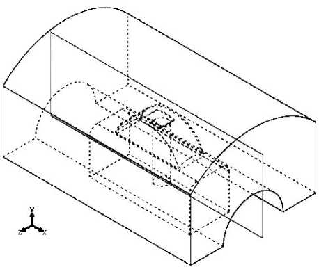
Fig. 1. The geometric model of the OMU

2.    Numerical Method for 3D Gas Dynamics Modelling

To solve the equations the volume control method, namely quasimonotone numerical scheme, is used. This method is a modification of the circuit S.K. Godunov [8-10]. Volume control volume are based on application of the Gauss - Ostrogradskv theorem. According T to this theorem for the vector field Ф = ( ф 1 ф2 ф3 ) and a closed volume V, wich is bounded by the outer surface S with the normal vector vecn, the equality is fulfilled div Φ⃗ dV =

Φ ^⃗ · ⃗n dS,

V

S

Φ=

where the divergence of the vector field in the Cartesian coordinate system have div дфXi;. According to (1), for the system of equations [1] and each index number corresponding to the equation system integrals over the volume of the control of non-viscous and viscous streams may be converted:

III (f + dG j ∂x ∂y V	+ ““ д”^ dV = ^ L j ' ndS = L j , S	(2)
fff (f j + G ∂x    ∂y	+ ^Hf) dV = fM ^ ^ = M j ,	(3)

VS where the components of the vectors of vicous flows Fj, Gj, Hj, standing consistently in every j-th equation systems are joined into the vector Lj = ( Fj Gj Hj ) T. and the components of the vectors of viscous flows Fvj, Gvj, Hvj, facing successively in each J-th equation systems are joined into a vector Mj = ( Fvj Gvj Hvj )T. Thus, change of the vector of conservative variables in each cell is defined by flows across the border, and by sources / sinks in volume, which are defined by volume integrals from source component members in vector. The numerical scheme is reduced to the assumption that the distribution of variables within a cell, finding flows through the faces of the cells and the integration time.

The differential-difference representation of the original system equations written for the calculation of the cell is given by:

d qq ( t ) + R ( t ))

dt

v []l ^L f-i ^{+ M} f-i

where V is cell volume, L f i is flux thro ugh the face F i, corresponding to the formula (2), M f i is flux through the face of f i, according to the formula (3), the summation carried out on all limiting the cell faces;

^{q (} t >=У

q ( x, y, z, t ) dxdydz

is average over the entire volume of the cell value of the vector of conservative variables q at time t. The value averaged by the cell volume of source members is determined by a similar formula. R ( t ).

Fig. 2 presents the types of cells that are valid for conducting numerical experiments. Splitting the computational domain into control volumes should be carried out in such a way that adjacent cells together had only one common face. Thus, the number of adjacent cells is determined by the number of cell faces. Cells having a common face each other, are called adjacent.

Splitting the computational domain into control volumes should be carried out in such a way that adjacent cells together have only one common face. Thus, the number of adjacent cells is determined by the number of cell faces, and cells having a common face are called neighbors. Non-viscous flows on each face of the control volume (cell) corresponding to the equations of conservation of mass, momentum and energy, are calculated using the approximate solution of the Riemann problem, namely by the method AUSM-M (AUSM -advection upstream splitting method [4]). AUSM-methods for calculating viscous flows are quite economical and suitable for calculating viscous flows. At this move to a coordinate

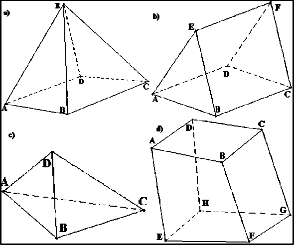
Fig. 2. Types of acceptable computational cells (control volumes): a) the pyramid ABCDE, which lies at the base of arbitrary the quadrilateral; b) a prism ABCDFE formed as a result of pulling (parallel transport) along the triangle ABE a side edge, such as along BC; c) the tetrahedra ABC; d) ABCDEFHG hexagons which edges are arbitrary the quadrangles

system is associated with the face and we consider only the part of velocity which is perpendicular to the face, sensing tangential velocity as a portable scalar. We get a vector of flow

/ pu) puu + p ρaM ρuaM ft*/ ( 0 j p F= pvu) = pvaM + 0 ,                           (6) pwu) ρwaM 0 phu) ρhaM 0 where h = e+p is gas enthalpy, u is the projection of velocity on the direction normal to the face (u = uin^. Values p, u, v, w, h are are considered as passive scalars transported by convective speed M and rely equal to the corresponding values from the "left" cell if the convective velocity on a face directed toward the "right" cell and vice versa. Value p) represents the action of the pressure.

Thus, due to the fact that convective and acoustic speeds are different, the flow F is the sum of two components. M is the Mach number obtained in AUSM-M method as the sum of the "convective velocity", partly coming from the "left" ( M + and partly from "right" ( M— ce 11 ( M = M ^ + M—. Part of the flow vector, associated with pressure, is also decomposed into the sum of two components from the "left" (P+) and "right" (P — cell in dependence of the Mach numbers and pressure in these cells ( p = P ^ + P—.

The splitting of the Mach number and pressure is carried out using the following:

M±     \ _ { ^ 4 ^{( M} ± 1) ^,

I M | <  1 ,

I M | >  1 ,

ML/R(M ) = | 2 (M ±M |), р± (Мп} = [ ±4 (м ± 1)2 (2 Р M) ,      IM| < 1,

L/R ^{( ,Р}) \ p (M ±IM I )/ M,            I M I >  1 .

Under the assumption of a constant distribution of the parameters within the cells method is only the first order accuracy in space. To achieve the second order accuracy is used piecewise-linear recovery, that is, within a computational cell is assumed linear distribution of the physical parameters. In this case, vectors of variables on the left and right faces of the cell, which separates adjacent cells with numbers textit i and textit j, necessary for solve the problem of decay of a discontinuity can be defined as follows qL = qi + Vqi • rL qR = qj + Vqj • rR ,

where q is a scalar variable, Vq - gradient and the variable r is a vector extending from the center of the cell in the center of the face.

It is well-known that the recovery of the second or higher order requires the use of limiters for suppressing artificial oscillations of solutions in the fields of high gradients. We use Barth and Jespersen limiter, specially designed for unstructured meshes. The value of the limiter in each cell is selected as a minimum limiter value determined for each face which bounds the cell. The value of the limiter for the face in this embodiment is determined by the condition that the values on the face do not exceed the maximum and minimum values in the cells of the whole pattern, consisting of counterflow cell and all its adjacent cells. The resulting limiter is of the form:

W =

<

Ф

-

max( q N ,q p ) - q p Vq p • (r f - r p )

, q f > q P

_ф q p - ^min( q N , q p )

^Vq p • ⁽ r f - r p )    ^,

1 ,

q f < q P

q f = q p ,

where function Ф ( x ) = min( x, 1), inclex f corresponds to the value on the face of the cell, P corresponds to the opposite cell. N corresponds to neighboring cells of P. r f -corresponds to the radius vector of the center faces, r_p corresponds to the radius vector of cell center P. Then, for the value of limiter for cell P we have:

^_p = min ( ^ f ) .

After determining the value of the limiter for the cell, gradients, required for the linear recovery in the calculation of flux through the faces, are multiplying by the limiter value found for the corresponding cells.

To calculate gradients the least squares method is used. From template, which includes some current cell C and adjacent to her cell nb, is held hyperplane that restores distribution of a quantity Q within the cell with the maximum order of accuracy:

a ^{( C} ) q x

( C )

q y

( C )

q z

E nb ^A x lb E _nb A X nb A y nb E _nb A x nb A z nb

Enb AXnb Aynb n^A AXnb A Znb Enb Aynbb    Enb Aynb Aznb nb AynbAznb       nb Azn2b

E _nb A q nb A X nb E nb ^A q nb ^A y nb ^E _nb A q nb A z nb

П7

where A X nb = X nb - x c- A y nb = y nb - y c- A z _nb = Z nb - z c- A q nb = q nb - q c- the slope of the plane corresponds to the required values gradients within the cell ( q X^c ) = d^ | _c,

(c) _ dq qy  = dy c

( c ) _ ^dq

• qz = dz C¹'

The gradients of velocity and temperature, and turbulent values on the faces of the cells necessary to calculate the viscous flows may be calculated as the average of the calculated gradients of the centers of the cells:

^q f • n = 2 ( ^q L + ^q R ) •ⁿ-

However, it is known that such an approach can lead to a mismatch decisions on rectangular or hexagonal grids, so we use a modification of the formula [5]:

q j

^^q f •ⁿ = П

-

-

n L i & lr + 2 ( ^q L + ^qR ) • ( n - ® lr s ) ,

where n is normal vector to the cell face, s is normalized vector joining the centers of the cells. || r_R - r L I is the distance between the centers of the cells L and R. a_LR is the scalar production a_LR = s • n, index f corresponds to the value on the cell’s face.

For the time discretization we use the explicit Runge - Kutta method of the second-order accuracy:

i - 1

q? = El “ t q ” + e m A tL ” ], l = 1 , 2 ,-,P,                 (12)

m =0

which flows in the cell c are the sum of the convective and diffusive fluxes through the faces of the cell L Cm ) = L ⁽ q C^m ) ,q C”\ ,...,q_a ”[ ) + M ⁽ q C^m ) ,q C” 1 1 ,...,q_a ”[ ), while the indices of adj 1, ... , adj_n correspond to adjacent cells to the cell c (i.e., having a common face), the indexes l and m correspond to the temporary layer. The order of accuracy, as well as preservation TVD properties achieved by selecting an appropriate set coefficients a ” , e lm and method’s order p. The initial values in the method correspond to the respective values at the current time tⁿ. The final values obtained in the method correspond to the next point in time t ^{n +1} = t ⁿ + A t. We use Runge - Kutta method of the second order with the following set of parameters: p = 2, a ₁₀ = 1, в ₁₀ = 1, a ₂₀ = 1 / 2, a ₂₁ = 1 / 2, в ₂₀ = 0, в ₂₁ = 1 / 2. Time step A t is calculated taking into account the non-viscous and viscous restriction on the step size. Approximation of the system of the last two levels is carried out by the control volume method:

Iff dt(pk) - (Pk - pe + pD)dV = (dt(pk) - (Pk - p£ + pD)) Iff dV = VCVC

= И(-d(fu) - dy(pvk) - dz(pwk) + д((p + S)dx)+

+/(( p+й) dk) + £ (( p+st) g)) ds, where the second inequality is written by the mean value theorem. Then the equation has the form

Vol. -p

A t

-CONVn + DIF,n + Vol • Pk++1 - Vol • pen+1 ij            ij                kijij where Vol is the volume of cell VC, CONVin is the part of the equation responsible for explicit approximation of convective members, and DIFn is the part of the equation responsible for the explicit approximation of the diffusion members. The production of kinetic energy can be approximated explicitly Pknj1 ~ Pkj since the member dissipation of kinetic energy of the turbulence presents in the form of

^ n+1

- V o ^ ^Д t ^ ^ j •

-Vol ■ A t ■ p j _ -Vol • Д t • pj ■   '

kij

Thus, we have the equation for calculating kinetic energy turbulence in a new temporary layer

_{n            n}     DIF _i ⁿ _j - CONV _i ⁿ _j

+ 1   pkj + A t ^ \ к^Ч + Volr J n +1

.

ij             on+1 + A t ■ o— pij   ' ^ t p kn ij

Similarly, the equation for dissipation is approximated as follows:

n+1 _ bij   =

n

P^p + A t • T c. 1 f П, P    + ij

DIF _i ⁿ _j - CONV _i ⁿ _j

■ ' + A t •

V ol r n   εinj

TE c.2 f2ij p kn ij

)

3.    Assessment of the Airflow Impact on the OMU

The impact of time-varying air pressure torque on the OMU can lead to strong vibrations and even resonance oscillations of the OMU, that is totally unacceptable. Therefore, the time pressure forces defines the dynamic loading on the the OMU. The time pressure forces are calculated relative to the unit geometric center (Fig. 1).

Forces and torque are determined by the formulas:

NN

Fx _ E Fix _ EPiASinix, i=1

NN

Fy _ EFiy _ EPiASiny, i=1

NN

Fz _ EFiz _ EPi ASiniz, i=1

⃗ ^N

⃗

M _ E^ i ^X F i ,

i =1

where the summation is over all the wall cells, p i is the pressure in the parietal cell, A S i is a surface element (along the solid surface), on which the force acts, n _ ( n_ix N_iy n_iz ) is a unit normal vector to the surfaces. Because of the symmetry F_z _ 0. -t is the radius vector drawn fr( m i the center of the the OMU t(:> the area, middle of the unit. F i is local pressure force ( F i _ ( F_ix F_iy F_iz )). Due to the symmetry the problem remains the only component of the torque about the axis Z.

Because of the symmetry with respect to the xy plane of the coordinate system (Fig. 1), corresponding components of the air pressure torque are equal to 0. The change in time of Z component is shown in Fig. 3.

The time interval corresponds to approximately 0,08 s time transients in the calculation scheme. Dynamic loading on the OMU is negligible, of the order ± 60 N • m. However, even such a small stress can result in significant impacts on the unit in the event of resonance. The impact of pressure forces on the OMU should be simulated to analyze the drive dynamics on the possibility of resonance.

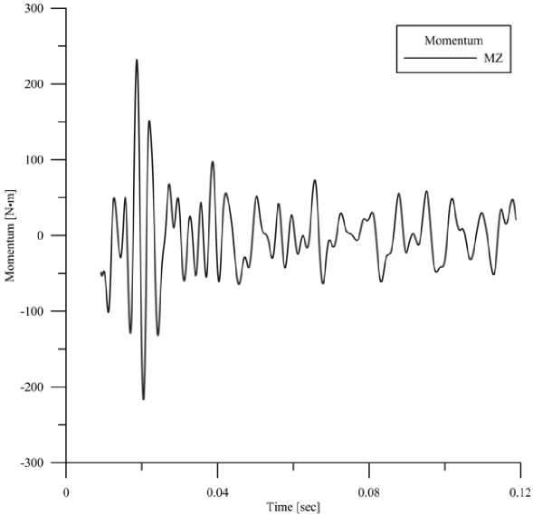
Fig. 3. The torque about the OMU center. MZ is the component of the torque along with the z axis direction, time is in seconds ( ж -axis), torque is in N ■ m (y -axis)

4.    Description the Simulation Algorithm

Theoretically, the proposed gas-dynamic model in the presence of the required computer capacity allows you to simulate the impact of airflow on the OMU with any given accuracy. But when you run a simulation on the proposed gas dynamic model, the computation time for the simulation was about 24 h per one period of oscillation at a frequency of 50 Hz. Using time series, it was found that for the end of the transition process in at simulation requires at least 0,1 s. It is clear that to carry out the simulation of gas dynamics for a few seconds is almost impossible. It is therefore proposed to use the short time interval to simulate gas dynamics and to use its results to build stochasticprocesses.

The proposed algorithm simulation:

• 1.    We form geometric model of the OMU, including a platform, a output window in the fuselage and a protective radorn.

• 2.    We simulate the airflow impact on the OMU using gas dynamics for a limited time interval that is determined by the transition process and generate the output data in the form of time series of the resultant force and torque in the OMU’s geometriccenter. The number of selected points in time series is restricted only by the required volume for storing files. Those time series are considered as some trajectories of stochastic processes. Simulation time interval is determined by the time of transients in the implementation computing circuit and computing time.

• 3.    The obtained time series of the resultant force and torque are used to estimate spectral and correlation characteristics of stochastic processes.

• 4.    We develop stochastic model to simulate the airflow impact on the OMU. On the basis of estimates of spectral and correlation characteristics we develop shaping filters for stochastic processes mathematical modelling.

• 5.    We perform mathematical modelling of the airflow impact on the OMU at a predetermined time interval.

It should be noted that using of the stochastic model of the airflow on the OMU reduces the computation time by several orders compared to the gas dynamics.

Conclusion

This article describes an approach to 3D mathematical modelling of the airflow impact on the optical-mechanical unit (OMU), mounted in the aircraft’s fuselage. The mathematical gas-dynamic modelling algorithm and stochastic models are used. In the proposed approach the gas dynamic model is used to retrieve the source data for constructing a stochastic model of the airflow impact on the OMU. Stochastic model is usefull for to express analysis of various design and technological solutions in the OMU’s development with moderate usage of computer time. The numerical 3D gas dynamics solution is presented, airflow impact assessment on the OMU is presented.

Acknowledgements. This work is conducted with the support of grant № 16-38-60185 and of the grant № 16-01-00fffa and of the grant № 15-08-02833a.