Mathematical terrain modelling with the help of modified Gaussian functions

The need to ensure the effective operation of all divisions of the Ministry of Emergency Situations (Russia) makes it expedient to develop adequate mathematical models related to possible catastrophes. Large flood is one of the main natural phenomena causing significant losses to the country’s inhabitants [1,2]. Large floods can be caused both by meteorological conditions and by the destruction of technical facilities in the inland water bodies. The prognostic modelling of the relief of reservoir basin bottom is actual. The considered problem is the predictive modelling of the water basins bottom topography, along with the modelling of flooded coastline relief to determine the water mass and estimate the possible flood consequences.

The use of Gaussian functions for the modelling of various surfaces is well presented in the modern literature [3–9]. In order to determine the numerous parameters of the flooded surface model, computer algorithms are usually used [4–7]. The target function is considered to be the root-mean square diversion from the empirical data of the depth measurement of the simulated basin terrain [7].

In this paper, we construct a model of two terrain sections: 1) a terrain model of the abovewater (coastal) section and 2) a terrain model of the underwater section. In order to construct the terrain models, we implement the following scheme. First, based on the normal distribution, we construct the localized Gaussian surfaces. Second, based on the empirical data of the pool depth measurement, we calculate the parameters of the localized surface section. Finally, taking into account the geographic and landscape features of the region, we construct a complete model on the basis of the localized Gaussian surfaces. We give the mathematical validation of the model equation choice as follows. First, we verify the statistical hypothesis about the possibility to apply the modified Gaussian functions in order to simulate both the abovewater and underwater sections. Then, using computer simulation, we improve the parameters of the model, which is the sum of modified Gaussian curves with the expected level of flooding. In fact, in order to simulate the convex and concave sections of the bottom surface, we use the stochastic modelling method.

In this work, we approach the terrain modelling in different ways. Namely, the mounds and cavities of the bottom relief are replaced by localized Gaussian surfaces closest to the real surface in the stochastic sense. Therefore, the locality of the extrema remains. Slopes surfaces are simulated by the equations of planes, the construction of which uses coordinates of the depth measurement points. This fundamentally new approach significantly reduces the number of model parameters. In addition, the model, as a functional form, can be used for various purposes of the Ministry of Emergency Situations (Russia).

In order to construct the model of the abovewater section of relief, we use horizontals of the topographic map.

1.    Statistical Hypothesis Verification

Note that the linear operations of ellipse reduction to the canonical form transform the two-dimensional distribution density to the following form:

1 1 X ² Y ² 1 X ² 1 Y ² _{2πσ x σ y} exp - _{2 σ x 2} + _{σ y 2} = √ _{2πσ x} exp - _{2σ x 2} ·√ _{2πσ y} exp - _{2σ y 2}

.      (1)

The right side of (1) shows that we have a product of two one-dimensional Gaussian curves. Therefore, in order to verify the statistical hypothesis of the type of distribution, we can use sections.

The results of the measurements were processed by the standard program shell Mathcad for the Pearson’s agreement criterion. For completeness of the presentation, we give the obtained computations below.

Based on the first section, we obtain that the number of depth measurements is n = 100, the number of intervals determined by the Sturges’ formula is 7, the minimum and the maximum depth measurements are 130 and 167, respectively, the average value is x¯ = 150, and the depth measurement procedures were carried out along the interval 4 · σ x = 4 · 6,2 ≈ 25m with the use of the analogue of the Two Sigma rule. Based on the second section, we obtain that the number of depth measurements is n = 50, the number of intervals is 6, the minimum and the maximum depth measurements are 142 and 167, respectively, the average value is y¯ = 150, and the depth measurement procedures were carried out along the interval 4 · σ y = 4 · 4,9 ≈ 20 m with the use of the analogue of the Two Sigma rule.

The measurements were carried out using rectangular carrier with the size 25 x 20 = 500 m 2 . Along the first section, the critical point is x kr = 12,28. The observed value of the criterion is х П_аЬ1 = 2,07. For the second section, we have that x kr = 11,37 and х П_аЬ1 = 5,01. In the both cases, the inequality χ ² _nabl < χ ² _kr holds. Therefore, there is no reason to reject the hypothesis of normal distribution.

2.    Localization of Gaussian Surface

Consider a two-dimensional Gaussian surface. Let xc , yc be the coordinates of the center of the surface, σx , σy be the root-mean-square deviations, and ρ be the correlation coefficient. Then the two-dimensional distribution density of the normal distribution has the form

1 f (x,y) =----------. exp

2na x ^ y ^ 1 - p ³

(<

- X c ) 2 σ x ²

2(x - X c ) ² (y - У с ) ²    (y - У с ) ²

p ----------------⁺----7---

σ x σ y              σ _y ²

Let us cross surface (2) by the plane z = z ₀ , which is parallel to the plane OXY . We obtain an ellipse in the section (Fig. 1). The equation of the projection onto the plane OXY has the form

(x - X c ) ²

x

-

²⁽ x ^- X c ^{) 2 (} y ^- У с ^{) 2     (} У ^- У с ^{) 2}     ,2

p --।--;----= d ,

σ x σ y               σ _y ²

where d2 = -2(1 -p2) In [2nz0axay ^T-p2]. In order to draw a section through the point M(xc + 2ax,yc), we apply the Two Sigma rule. At the point M(xc + 2ax,yc), the height of surface (2) is

----' xp . 2      = M (2). 2na x a y y1 - p ²

Definition 1. The part of surface (2) located above the ellipse is called the localization of the Gaussian surface

(x - X c ) ² σ x ²

-

_p 2(x - X c ) ² (y - У с ) ² + σ x σ y

⁽ У ^- У с ) ²

σ y ²

Besides neglecting 5 – 7% of accuracy, we localize the significant part of the surface by replacement of the elliptical carrier with a rectangular one.

The rectangle D _E is constructed such that ellipse (3) is inscribed in D E (Fig. 1). The practical application of the Gaussian surface is justified by the fact that the Gaussian surface is completely determined by the parameters. Namely, the parameters σ x , σ y determine the semi-axes of ellipse (3), and the parameter ρ determines the angle of inclination α of the axes of the ellipse symmetry (Fig. 1) by the equation

- 2(1 - p ² ) In ^nz o ^ x a y ^ 1 - p ² ] . (3)

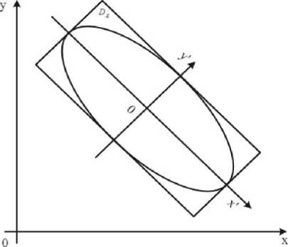
Fig. 1. Replacement of the elliptical carrier with the rectangular one

p=

σ ² σ ² xy

2a x a y

tg2a.

Denote the coordinates of the center of the rectangle D E by x c and y c . The center is the surface top. Since we chose the carrier according to the Two Sigma rule, the dimension of the rectangle is la x x 4a y . According to formula (4), the inclination angle of the new axes allows to determine the parameter ρ. This rectangle is the carrier of the model component. In addition, the surface height is inversely proportional to the region of the carrier

H„         8     • n^1 - P2  SDe

.

The indicator function of the rectangle D E is

„Е<Х.у>={

0, if (x,y) E D e ;

1, if (x,y) / D e .

The equation for the localized surface is fDe (x,y) = Pf (x,y XXEE (xy)

The part of the general simulated convex upward surface deviate from the normal distribution by the factor p >  0 (Fig. 2), and the equation for the part of a convex downward surface deviates from the normal distribution by the factor µ <  0 (Fig. 3). The constants µ are determined from the empirical sample at the point with coordinates (x _c , y c ) and characterize both the height of the underwater relief cap above a certain depth level and the depth of the underwater relief cap below a certain depth level. Similarly, we construct a model of the abovewater (coastal) section of the relief.

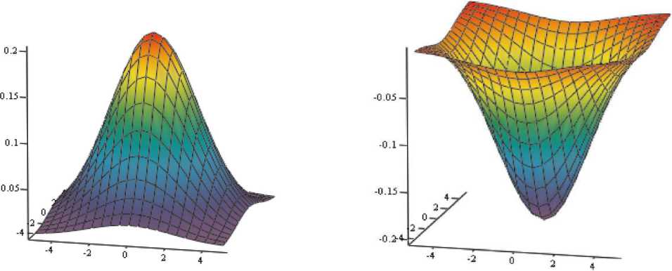
Fig. 2. Localized section of the surface (p> 0) Fig. 3. Localized section of the surface (p< 0)

3.    Determination of Parameters by Empirical Data

In [7], the empirical level lines are obtained with the help of empirical data on the depths of the investigated reservoir (Fig. 4 on the left).

In Fig. 4 on the left, solid lines indicate the average empirical level lines defining the convex sections of the bottom relief, and dotted lines indicate the boundaries (i.e. the cavities between them). It follows from the property of the normal distribution that the region of a rectangular carrier automatically determines the height of the bottom relief mounds or the depth of the cavities.

N = 8

N = 4

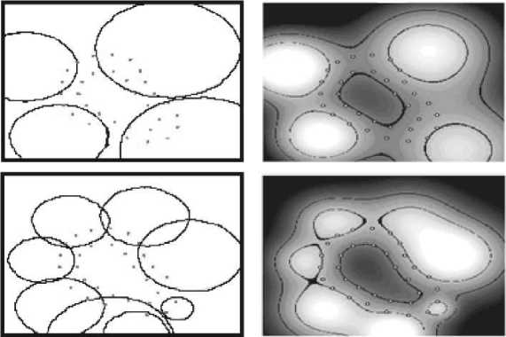
Fig. 4. Elevations (mounds) of the bottom relief are indicated by white color, and black dots indicate the cavities

The following statement gives the principal (stable) solution to the rectangle decomposition problem of the investigated region.

Theorem 1. [7] Every open non-empty bounded set on the plane is the union in pairs of at most a countable family of the closed rectangles without common interior points.

Taking into account the hydrological features of the edge of the water body under study, we obtain that the fine partition by rectangular carriers is impractical. If the depth line map of the reservoir is absent, then depth measurements are conducted, based on which the empirical level lines are constructed, the transitions between mounds and cavities are determined, and the size of the rectangles with provision for the depth difference are taken into account. In this case, we have a purely computer problem on determining the coordinates of the vertices of the rectangle associated with the empirical line of the depth transition level (Fig. 5).

4.    Statement of Computer Problem

Fig. 5 shows a scheme of the arrangement of depth measuring points on the empirical level line. The coordinates of the depth measurement on the line are given. It is necessary to determine the shape and position of the rectangle bounded by the given level line. More precisely, we need to determine (based on the given points) the coordinates of the vertices of the rectangle using a computer method.

We allow some certain simplifications in the model construction. In fact, these simplifications have little effect on the accuracy and reliability of the model, since we can change the number of carriers and replace a region with two adjacent ones.

Suppose the following.

• 1.    For the given carrier, the surface formula is unimodal.

• 2.    The region bounded by the horizontal is assumed to be convex. In other words, this region entirely contains any straight line passing through two points that belong to the region.

• 3.    The depth measurements were taken with a certain constant step. Therefore, the horizontal line can be replaced with the inscribed polygon.

  

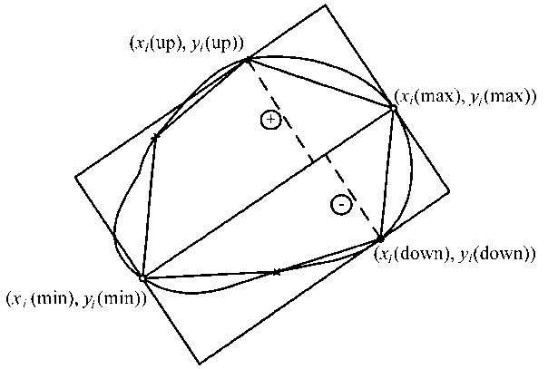
  Fig. 5. Construction of a rectangular carrier

  
  

Algorithm to determine the coordinates of the vertices of a rectangle.

• 1.    Replace the convex region with a polygon having vertices at the depth sounding points (x i , y i ) i = 1, 2, • • • ,m.

• 2.    Compare distance between all points and find two points located at the greatest distance from each other. Suppose that these two points have the coordinates (x i (max), y i (max)) and (x i (min), y i (min)). Find the equation of the straight line passing through these two points. Find the equations of two straight lines that are perpendicular to this line and such that the first line passes through the point (x i (max), y i (max)), while the second line passes through the point (x _i (min), y _i (min)).

• 3.    Compare the positive deviation of all points from the straight line passing through the points (x i (max), y i (max)) and (x i (min), y i (min)). Define the point with the greatest positive deviation (x i (up), y i (up)) and the point with the greatest negative deviation (x i (down), y i (down)) (Fig. 5).

• 4.    Draw two lines such that each line passes through either the point (x i (up), y i (up)) or the point (x _i (down), y _i (down)) and is parallel to the straight line passing through the points (x _i (max), y _i (max)), (x _i (min), y _i (min)).

• 5.    The pairwise intersections of the four lines described above define the coordinates of the rectangle vertices. Denote these points by (x 1 (p),y 1 (p)), (x ₂ (p), y ₂ (p)), (x ₃ (p),y ₃ (p)), (x ₄ (p),y ₄ (p)) in the counter clockwise order.

Based on the vertices of the rectangular carrier, we can determine all parameters of the Gaussian surface for which this rectangle is the carrier as follows.

1.    Coordinates of vertex are xc = xi (max) + xi(min) , Ус = yi (max) + yi (min) . 2. Parameters of the semi-axes of the ellipse ^x = 4 x/IxiCpT-^s(p)]2+Iyi(p)—^sCp)]2, are ^y = 4 VfMP) - x4(P)]2 + [У2(р) - y4(P)]2. 3. The parameter ρ is known from formula (4), and the angle is found from the following equation: yi(max) a = arctg xi (max) - - yi (min) xi(min) 5.    Modelling of Relief Slopes of Water Basin Bottom That Do Not Belong to Mounds or Cavities

Such slopes include the coastal zone, as well as the section of the intermediate zone between the cavities and the mounds (Fig. 4, 7). The land relief zones include the following: a lowland, a sole, a mud hole, a cliff, a section of a valley, etc. These sections are simulated by the definition of the plane equation. Let us consider the region bounded by the points of depth measurements (Fig. 6).

Let M(x, y, z) be a variable point on the plane (abkm) (Fig. 7), where the coordinates of the points are as follows: a(x 1 ,y 1 , 0), b(x ₂ ,y ₂ , 0), c(x ₃ ,y ₃ , 0), d(x ₄ ,y ₄ , 0), m(x ₃ ,y ₃ , - h), k(x 4 ,y 4 , - h).

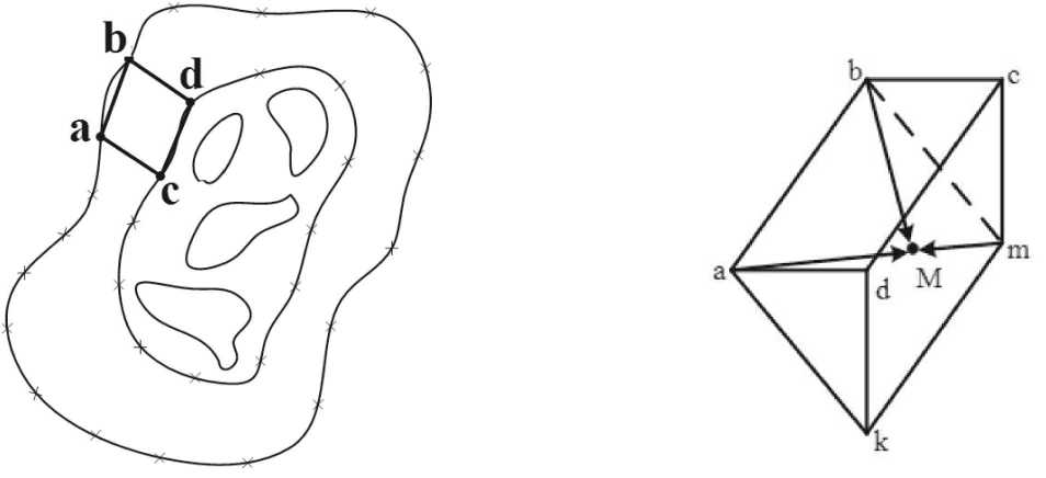
Fig. 6. An example of the region bounded Fig. 7. Construction of the plane by the depth measurement points

The equation of this plane is obtained from the vector coplanarity condition. The mixed product is ^aM, bM, mM^ = 0.

Calculate the determinant

x - x 1 x - x 2	y - y i y - y 2	z z	= 0,
x - x 3	y - У з	z + h

and obtain the equation of the plane

/ x       h(y 2 - y i ) ,    h(x i - X 2 )  ,   h(x i y 2 - y i X 2 )

z = p(x, y) = x-------+ y-----j--1---7------- dd  d

The region of the relief with a carrier in the form of a quadrangle P = (abcd) is simulated by equation (5) acting limited on the carrier:

P ^{( x,}y ) x X p_e ^{( x,}y).                                      (6)

Here x _P E (x, y ) is the indicator function of the rectangle:

X p_e ^{( x,}y ) =

{0

if ^{( x,}y) e P E ; if (x,y) / Pe .

Summarize all such sections and obtain the functional description of the relief zone considered in this paragraph:

P j (x^ ^x X p _e, (^y)

j ^j

Such a modelling can be used in the cases with a flat bottom or a plateau (Fig. 8).

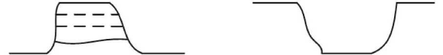
Fig. 8. Relief with a flat bottom or a plateau

6.    Complete Mathematical Terrain Model

The main problem of the flooded surface modelling is to predict the excess volume of water caused by natural or climatic weather conditions. For that kind of prediction, it is desirable to have a model with a certain small set of parameters that characterize the volume of water. Let h _{D j} be the depth on the level line corresponding to the rectangle D j (at the point (x _i (up),y i (up))), f j (x,y ) be the function defined by formula (2) for a given medium, (x j ,y j ) be the center of the carrier, and h(x j ,y j ) be the depth of measurement at the point (x j ,y j ). Then the equation of the mathematical model concentrated on the rectangle for the underwater mound is as follows:

F D j ^{( x,}y) = ^v + ^x

M ^{x f} j ^{( x,}y)X Dj ^{( x,}y )

where m = - 1, v + = \h_Dj - h(x j ,y j )].

The equation of the mathematical model concentrated on the rectangle for an underwater cavity is the following:

F D j ^{( x,}y) = ^v - ^x [m ^{x f} j ^{( x,}y)X Dj ^{( x,}y )] ,                        ⁽⁸⁾

where m = +1, v - = hhx j j ,y j ) — h j .

The complete equation of the section of the flooded relief is composed of all local functions calculated for the cavities and mounds (7) – (8), and the volume concentrated on the sections of the bottom relief simulated with the help of planes (6):

F water section = 52 ^F D j ⁺ 52 ^F D j ⁺ 52 P j ⁽ x, у) ^x X pj ⁽ x, у) '              ⁽⁹⁾

jjj

A similar approach is used to construct a land-based relief model for the coastal zone. A map of the level lines is used to determine the size and location of the rectangular carriers of the model of the abovewater coastal section of the landscape.

Conclusion

In this work, based on a fundamentally new approach, we obtain a complete mathematical model of the flooded terrain. Nevertheless, over time, especially the water

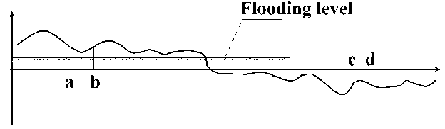
Fig. 9. Flooding level line section of the model can change. In this case, a new model can be constructed by the proposed technique. Note that the current technical level of echosounders allows to use the echosounders in order to determine the level and shape lines of the water carriers. In order to construct a surface model, other approaches are possible, for example, digital modelling and mathematical simulation with the help of a high-order polynomial [10, 11]. In this case, there exist both the difficult problem on determining a large number of coefficients of a polynomial surface and the need to calculate a large inverse matrix. It is known that this problem is laborious and has relatively wide margin of error.