Modeling of a closed mono-branch labor market conditions

The role of able-bodied citizens in economy is significant as labor being one of the production factors is the economy “foundation” or basis. Studies devoted to the dynamic processes of a labor market are currently acute as the phenomenon is investigated by both Russian and foreign scholars [1–7]1.

The purpose of the study is to construct a closed mono-branch mathematical model that reveals the staff dynamics features in terms of labor market conditions.

Different studies are devoted to this issue. Several dynamic stochastic models of general equilibrium were considered [8–10]2, as well as econometric models of the labor market as an element of a macroeconomic system [11–13]. A well-known model developed by C. Shapiro and J. Stiglitz [14] also considers a staff classification according to salary rate and labor productivity. And production functions are used as modeling tools in most of the studies.

From the Russian-language literature on the issue under consideration, we note the publications by A. Vasil’ev, where a onedimensional differential model of the labor market was proposed [15]. Later it was transformed into a multidimensional system by I. Zaytseva [16]. A. Golyatin [17] was also engaged in forecasting the dynamics of the labor market using the apparatus of systems of differential equations. However in all the above mentioned studies the mathematical model has not been derived from basis prerequisites, which makes it impossible to assess the scope of the model and the possibility of its generalization.

In this connection we firstly designate the labor market conditions, which represent a complicated dynamic system. The laws of its functioning will give grounds for adopting the hypotheses that define our model.

The main elements of the labor market system are its subjects. The subjects of the labor market, as well as those of any market, are a seller and a buyer. In the considered case they are an employee (a worker) and an employer, respectively. The interaction of employers and workers in the labor market as a whole determines its condition, which is the ratio of supply and demand.

The labor market conditions depend on the state of the economy, the branch structure of the economy, the level of technical basis development, welfare of the population, the development of the market of goods, as well as on services, housing, securities, the state of social and industrial infrastructure, the development degree of the multistructure of the economy, and measures for the development of integration ties [18]3. It can be of three types [5; 19]:

• -    labor-deficit, when the labor market lacks supply of labor (this state of the labor market is usually accompanied by extremely low unemployment);

• -    labor surplus, when there is a large number of unemployed in the labor market, and the level of labor supply exceeds the level of its demand;

• -    equilibrium, when the demand for labor corresponds to the supply.

Dynamic processes of labor market conditions arise due to the complementarity of the interests of a job seeker and an employer. Any job seeker aims to find a job, while the employer's goal is to increase the efficiency of activities of the firm by employing highly qualified personnel and getting rid of workers who do not meet the requirements of the enterprise.

Proceeding from these premises, we may divide all economically active subjects of the labor market in any particular field of activity into three categories:

• -    highly qualified specialists are specialists with specialized education and experience in the field of activity. They are those in whom the employer is primarily interested;

• -    specialists of the intermediate level have a potential to become highly qualified specialists in the field, but there is no guarantee of realizing this possibility. The employer is interested in distinguishing from this category subjects who can really become specialists of the high category;

• -    low-level specialists do not even have a potential to become highly qualified

specialists in this field, the employer not interested in them.

The purpose of the study is primarily the optimization of work with personnel. It is the labor market conditions as a paradigm of dynamic processes of the market that are the subject of the study. The transition from qualitative analysis to quantitative analysis is carried out by means of a mathematical model, which is constructed as described below.

Mathematical model construction

We represent the labor market in the form of two disjoint sets: employed citizens and unemployed ones. Each of these sets is divided into three (also disjoint) subsets, which we identified above as specialists of high, intermediate and low categories. The number of elements in each set is measured in general conditional units (tens, hundreds, thousands, etc.).

We accept the following hypotheses:

• 1.    The total numbers of employed and unemployed citizens are constant in time;

• 2.    The total number of subjects of each category in the labor market is known and constant;

• 3.    Rational behavior of the employer towards specialists of the high category implies an unconditional desire to increase the number of them in the enterprise;

• 4.    Rational behavior of the employer towards specialists of the low category implies an unconditional desire to reduce the number of them in the enterprise (complete exclusion is ideal). Therefore the positions occupied by low-level specialists are a priori considered to be vacant.

As to specialists of the intermediate category, the enterprise makes selection between them, with a part of them accepted for work as a result. The enterprise can exert a significant influence on the process of differentiation of the intermediate-level specialists (the so-called ”training factor” will be introduced below).

Based on the above hypotheses, it is already possible to make reasonable qualitative assumptions about the dynamics of each of the categories of labor market subjects. For example, it is obvious that the number of specialists of the high category in the enterprise will increase permanently, while the number of specialists of the low category will decrease. However, heuristic estimates are not enough to give a prognosis about the quantitative correlation of the subjects of the labor market in the enterprise. Such a description can be given only by a corresponding mathematical model. Now we pass to constructing it.

In the model we suggest let М be the total number of employed citizens, N be the total number of unemployed citizens, A be that of specialists of the high category at the labor market, B be that of specialists of the intermediate category, and G be that of specialists of the low category.

Further, let a_M (a_N ) be the fraction of specialists of the high category in the total number of employed (unemployed, respectively) subjects; в_м (вы) ^_ the fraction of specialists of the intermediate category in the total number of employed (unemployed) subjects; Ym ( Yn ) ^_ the fraction of specialists of low category in the total number of employed (unemployed) subjects.

The total number of subjects in each of the categories is described by the product of the number of subjects in the sets of employed and unemployed citizens by the corresponding fraction (Fig. 1).

Employed specialists ( M )
High category ( a M М)	Intermediate category ( P m М )	Low category ( У m М )
Unemployed specialists ( N )
High category ( a n N )	Intermediate category ( P n N )	Low category ( У n N )

Fig. 1. The number of subjects in the categories of labor market subjects

Each of the categories of subjects among employed and unemployed subjects is a function of time. Our purpose is to find the dynamics of the introduced above functions a m , a n , P m , P n , у m , у n , that is to find the law of the variation of them in time. However, above all we note that the following stationary relations are true for them:

First, it follows from the definition of the functions am (an), pm (pn) and уm (уn ) that a m (t)+ P m (t) + У m (t) =1, aN (t) + P N (t) + У N (t) = 1.

Second, from hypothesis 2 we have:

a M (t) M + a N (t) N = A,(2)

Pm (t)M + PN (t)N = B,(3)

у m (t) M + y n (t) N = G.(4)

As it was noted above the set of employed specialists of the intermediate category is divided into two subsets kM p_M ( _t ) and (1 - к ) m p_m ( _t ) . Subjects of the first subset leave the enterprise, while those of the second subset stay in it. Here by k the so-called training factor is denoted. It is not the same for all enterprises, but is an individual characteristic that shows the quality of personnel work in the enterprise. The smaller k is, the better personnel work. Decrease in k can be achieved in various ways: rapid and highly effective training, prospects for professional and career growth, material interest.

Fix two arbitrary moments of time t , t + A t , and find how the numbers of specialists of the high, intermediate and low categories are changing during the time interval A t .

Consider the dynamics of the function ^a m ⁽ t ) . Where t о and t о ^{+ A} t are two time moments. In that case ^a m ⁽ t о ) ^M is an amount of employed highly qualified specialists at the time t о .

Per unit time low-level specialists ^y m ⁽ t о ) ^M and specialists of the intermediate level ^{k P} m ⁽ t о ) ^M discharge; the vacancies they make are occupied by subjects who are unemployed at that time.

Since ^a n ⁽ t о ) is a share of highly qualified specialists in the total amount of the unemployed then, correspondingly, the share of jobs occupied by highly qualified specialists at the time ^A t is logically equal to their amount among the unemployed. Correspondingly, due to hypothesis 3 the amount of highly qualified specialists at t о ^{+ A} t is:

am (tо + A t) M = a m (tо) M + a n (tо) M (ym (tо)+кв m (tо))А t. Now let us consider the changes of the function Pm (t) at the same time period from tо to tо + At. The amount of the employed specialists of the intermediate level at tо is pm(tо)M .  Since  pn(tо)   is a share of specialists of the intermediate level in the total amount of the unemployed. However, the amount of specialists of the intermediate level who were discharged at the same time period should be subtracted. The amount of these people is kpm(tо)M. Thus, the amount of specialists of the intermediate qualification at tо + At is:

P m ( t о + A t ) M = P m ( t о ) M + [ P n ( t о ) M ( y m ( t о ) + к P m ( t о ) ) -- к P M ( t о ) M ] A t .

And finally let us consider the dynamics of the ^Y m ⁽ t ) function. The amount of the employed low-level specialists at the time period t 0 is Y m ( t 0 ) ^M . Since Y n ⁽ t 0 ) is a share of low-level specialists in the total amount of the unemployed then, correspondingly, their share in the occupied positions at the time period is equal to their share in the unemployed. However, the amount of the low-level specialists who were discharged at the time period Y m ⁽ t о ) М (according to hypothesis 4) should be subtracted. Thus, the amount of low-level specialists at the time period t о + A t is:

Y m ⁽ t о ^{+ A} t ) ^M = Y m ⁽ t 0 ) ^M + [ Y n ⁽ t 0 ) ^M ( Y m ⁽ t о ) + k P m ⁽ t о ) ) ^— -Y m ⁽ t о ) ^{M ] A} t .

Point t о has been randomly chosen, so index 0 may be omitted. Thus, the following equations that describe the dynamics of employees of the three categories have been obtained.

a _M ( t + A t ) M — a _M ( t ) M = = [ a n ( t ) M ( y m ( t ) + k в m ( t ) ) ] A t ,

P m ( t + A t ) M — в m ( t ) M = [ в n ( t ) M ( y m ( t ) + k в m ( t ) ) — — k в m ( t ) M ] A t ,

Y m ( t + A t ) M — y m ( t ) M = [ y n ( t ) M (y m ( t ) + k в m ( t ) ) —

—Y m ( t ) M ] A t .

Divide the both sides of each equality by A t , pass to the limit as A t ^ 0, and take into account equalities (2), (3), (4). As a result we obtain the following system of three differential equations with three unknown functions:

a M ( t ) = ^f A  ^— a ^{M (} - ) 'I ( y m ( t ) + k p m ( t ) ) ,

I     N     )

« P M ( t ) = f B — M MO ' ( Y M ( t ) + k в M ( t )) — k P M ( t ), Y M ( t ) = f G — M M ’l | ( Y M ( t ) + k в M ( t ) ) — Y M ( t ).

The second and third equations of system (5) do not contain aM, therefore they can be considered as an independent system with respect to two unknown functions вл/, Ym . The function aM is defined by them from the relation (1), hence the first equation of system (5) can be dropped, since it is equivalent to the identity (1). It remains to investigate the following system p —=f B—M^ h —+k в—)—k в — ■   (в»

Y — = ^   “ “M |(Y M + k в m ) — y m -

Then we construct an accurate analytical solution of system (6) and study its continuality and asymptomatic characteristics.

Solving the system of differential equation with given initial conditions

A ccording to the Picard theorem [20]¹ the system (6) with given initial conditions

в(0) = Po , y (0) = Yo is locally solvable, and its solution is unique.

As to analytic solutions, generally speaking, there are no universal methods for constructing them for nonlinear systems of differential equations [1; 20‒22]2. However, we will verify later that system (6) possess a number of useful properties, which make it possible to find its solution in quadratures.

For brevity denote M/N = m , b/n = b ,

G/N = g in system (6), and introduce new variables: твм = x, my m = y. We obtain the system

x = ( b — x )( y + kx ) — kx , _ч ^y = ( g ^— y )( y ^{+ kx} ) ^— y .

Obviously, system (7) has the trivial solution x (t) = y (t) = 0, which is by virtue of the uniqueness theorem is realized only for the initial conditions x (0) = y (0) = 0. However, if system (7) has a nontrivial solution, then at least one of the functions is different from zero in a neighborhood of the initial point. For the sake of definiteness we put y(t) > 0, since in case x(t) > 0 the consideration is analogous.

Multiply the first equation of system (7) by y , the second by x , subtract the second equation from the first one, divide the both sides of the resulting equation by y2, and denote xy = z. We obtain a first-order differential equation in separable variables1: z' = — kgz2 + (1 — k + kb — g) z + b.         (8)

The right side of equation (8) is a quadratic trinomial. Let us investigate its properties.     The quadratic equation

— kgz ² + (1 — k + kb — g ) z + b = 0 has the discriminant     d = (1 — k + kb — g )² + 4 kgb .

According to the physical sense of the problem, k >  0, g >  0, b >  0, therefore D >  0 , and the quadratic equation has two real roots:

1 — k + kb — g — -Dd    _¹~ k + kb - g + 4D   (9)

z ¹ =         2kg        ’ ²           2 kg         ■

Note that z_l <  z₂ and z ₂ >  0 . By the

Substituting x = zy into the second equation of system (7), where the function z ( t ) is defined by the equality (10), for finding the function y ( t ) we obtain a Bernoulli equation У + (1 — g — kgz ) y = — (1 + kz ) y ² .

Have solved it we find the function

y ( t ) , and also x ( t ) :

y ( t ) =

y 0 u ⁽ t )

y ₀ j (1 + kz ( s )) u ( s ) ds + 1

x ⁽ t ) =

y 0 ^{z (} t ) ^{u (} t )

t y 0 j (1 + kz (s)) u (s) ds +1

Vieta theorem, zz ₂ = — b/kg <  0 , hence z <  0 .

Here the function z(t) is defined by (10), c = z 0—z1 , and z 0—z 2

It is simple to verify that all solutions

of equation (8) have the form:

u ( t ) =

C — e " t

C — 1

_e ⁽ g ^— 1 + ^z 2 kg ) t .

z ⁽ t ) = •

X^      л—® t

Cz 2 — z 1 e

C — e " t

, если z 0 ^ z 2 ,

z ₂, если z 0 = z₂.

An arbitrary constant С is determined by the initial conditions, so C = z 0—z1 . It is z 0—z 2

obvious that C = 1 can be only in case z₁ = z ₂, which contradicts the properties of z₁ , z ₂. Hence the case C = 1 is excluded. Consider all the other cases.

• 1.    Suppose z ₀ >  z ₂. Then c >  1 >  e ““ t , the solution is defined for all t >  0, moreover,

• 2.    Suppose       z ₀ e ( z 1 ; z ₂).       Then

• 3.    Suppose z ₀<  z . Then C e (0; 1) . Hence there exists a point t ₀ >  0, where C = e ^_“ t ⁰ . The solution has a vertical asymptote t = t ₀, is uniquely defined in the interval t e [0; t ₀ ), moreover, z ( t ) <  z₁ . The solution cannot be extended to the set

z ( t ) >  z ₂ .

C < 0 < e “" t, the solution is defined for all t > 0, moreover, z (t) e (z1; z 2).

t e [ 1 0 , +w ) .

The above analysis of the function z ( t ) makes it possible to find conditions for extendibility of the functions x ( t ) and y ( t ) .

Suppose x ₀ >  0, y ₀ >  0 . Then z ₀ >  0 . Let us prove that in this case z ( t ) >  0. If z ₀ >  z ₂, then z ( t ) >  z ₂ >  0 . Now suppose that 0 <  z ₀<  z ₂. Find the derivative of the function z ( t ) defined by (10): _z '_{( t} ) = ^{( z} 1^{— z} 2 ) ^C " ^e " t

( C — e “" t )² .

In this case C <  0 , and since z₁ <  z ₂, we have z ‘ ( t ) >  0. It follows that the function z monotonically increases on the whole real axis. Hence in this case we also have z ( t ) >  0.

It follows now from formulae (11) that if x ₀ >  0, y ₀ >  0, then the functions x ( t ) and y ( t ) are nonnegative, continuously differentiable, and extendable onto the whole semiaxis [0; w ).

It should be mentioned that a solution constructed on a finite interval does not give reliable information about the behavior of the solution as the argument increases infinitely. Correspondingly the question of asymptotic behavior of a solution requires special investigation. We begin it from finding the equilibrium points1, which are stationary solutions of system (8) x(t) = x* = const,

y ( t ) = y* = const . These constants are the solutions of the following system of algebraic

equations: / b ^{x )( y} + kx ) kx = °,

, ( g - У )( У + kx ) - У = °.

It is easily seen that system (13) has three (and only three) solutions, which are the equilibrium points of system (8):

x * = 0 , y * = 0 ;

„* _ kgz + ⁽ g - 1) z i ,,* _ kgz i + ⁽ g - 1) ; ^x                         , ^y

1 + kz ₁                1 + kz ₁

* _ kgz 2 + ⁽ g - ^{1) z} 2   * _ kgz 2 + ⁽ g - ¹⁾ .

x^ =----------------, y о =-------------

1 + kz 2               1 + kz 2

Here z₁ , z₂ are the roots of the quadratic equation defined by formulae (9). Taking this into account, one can easily show that the second and the third equilibrium points possess the following property: x * + y * = b + g - 1, i = 1,2.

Let us find the limits, as t ^® , of the functions _x ( t ) and y ( _t ) defined by equalities (11). We begin with calculating the limit for the function z ( t ):

numbers x *" , y *' should be negative, which is impossible, because the functions x ( t ) and y ( t ) are nonnegative.

Replacing z by its expression, we obtain that the inequality g -1 + z2kg > 0 is equivalent to the inequality b + g > 1 (correspondingly,       the       inequality g -1 + z2kg < 0 is equivalent to the inequality b + g < 1). Thus, the results of the present section take simple and completed form:

• - If b + g <  1 , then lim y ( t ) = 0, t >x

lim x ( t ) = 0.

t ^X

• — If b + g >  1 , then   lim y ( t ) = y * ,

t ^X lim x (t) = x *.

t ^X

Phase portraits of system (7) in coordinates (х, у) are presented in Fig. 2, 3 . Fig. 2 displays an equilibrium point (0,0), whereas Fig. 3 - an equilibrium point ( x 2 , у * ) . Both equilibrium points are stable nodes according to the classification of the theory of

Cz л — z, e lim z ( t ) = lim — ²—¹— t ^x      t ^» C — e ^at

= ^z 2 .

Therefore, lim x(t) = z2lim y(t) • Thus t ^® t ^® the problem is reduced to calculating the limit of the function y(t) • This requires the analysis of the asymptotic behavior of the function u (t) defined by the equality (12).

Obviously,

lim t ^»

С - e ~^m ‘

C - 1

С

С - 1

hence

the asymptotic behavior of u ( t ) is defined by the sign of the constant g - 1 + z₂kg . It follows from equation (11) that the functions x and y tend to the third equilibrium value in case g - 1 ₊ z₂kg >  ° , and to the first (trivial) equilibrium in case g - 1 + z₂kg <  0 • The second equilibrium point is not realized in the model given. Indeed, since z_t <  0 , one of the

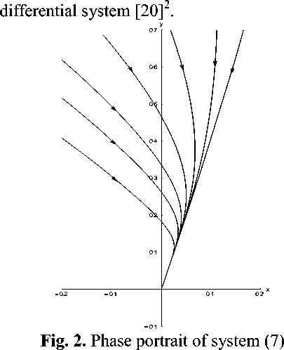
for the equilibrium point (0,0).

1 Demidovich B.P. Lektsii po matematicheskoi teorii ustoichivosti [Lectures on mathematical theory of sustainability]. Moscow, MGU Publ., 1998. 480 p. (In Russian).

2 Also see: Erenberg R.D., Smit R.S. Sovremennaya ekonomika truda. Teoriya i gosu-darstvennaya politika. Per. s angl. [Modern economy of labor. Theory and public policy. Trans. from Engl.]. Moscow, MGU Publ., 1996. 800 p. (In Russian); Demidovich B.P. Lektsii po matematicheskoi teorii ustoichivosti [Lectures on mathematical theory of sustainability]. Moscow, MGU Publ., 1998. 480 p. (In Russian).

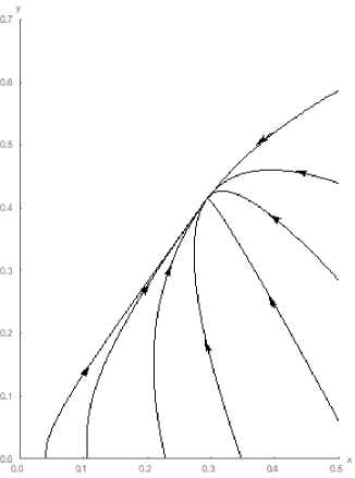
Fig. 3. Phase portrait of system (7) for the equilibrium point ( x * , у * ) .

Then we analyze the obtained results using the terms of the initial model and will economically interpret them.

Interpretation of the results in terms of the original model

T o interpret the results let us return to the above-mentioned notations: M N = m , B N = b ,

GIN = g , в m ( t ) = x ( t )/ m , Y m ⁽ t ) = У ⁽ t )/ ^m . Using these terms we reformulate the main results of the model construction.

System (5) possesses the following properties in any finite segment:

• -    For every initial conditions a₀ >  0 , P o >  0 , Y o >  0 ( a o +P o + Y o = 1) system ^{(5) is} unique solvable;

• -    The functions α _M , β _M , γ _M are

extendable to all the semiaxis [o, +w ) and are nonnegative;

• -    The solution of system (5) is presented in quadratures:

  Y m ⁽ t ) =

  
  

Yo u W

P m ( t ) =

t                                               ,

m Y o f (1 + kz ( s )) u ( s ) ds + 1

o

Y o ^{z (} t ) ^{u (} t )

t                                                 , m Yo f (1 + kz (s)) u (s) ds +1

o where the functions z (t) and u (t) are defined by the equalities (10) and (12) respectively.

The asymptotical behavior of solutions of system (5) is described by the following statements:

• 1.    If B + G <  N , then lim a _M ( t ) = 1,

• 2.    If B + G > N , then

t→∞ lim p m (t) = o, lim Ym (t) = o. t→∞

b + g - 1

lim am (t) = 1---—, lim pm (t) = t→∞           m    t→∞ lim y m (t) = У2.

In the first case, A+B+G=M+N≤A+N. This means that the number of specialists of the high category in the labor market is greater than the total number of workplaces. The dynamics of the functions a_M ( t ) , p^ ( _t ) , Y_M ( t ) is obvious: the fraction of specialists of the high category in the enterprise tends to 1, while the fractions of specialists of the intermediate and low categories tend to 0.

In this situation, on the one hand, the enterprise has the opportunity to maximize the efficiency of activities by employing exclusively specialists of the high category. There is no need to work with personnel. On the other hand, if a >  M , then some of the highly qualified personnel turn out to be unclaimed. As for specialists of the intermediate category, they have no chance to get a job, therefore, they loose motivation for self-improvement in this area. At the same time, the enterprise deprives itself of the opportunity to recruit potentially strong specialists of the intermediate category, since at this stage they cannot compete with specialists of the high category. On Fig. 4, 5 and 6, the graphs of the functions a_M ( t ) , P_M ( t ) and y_m ( t ) are represented for the first case.

^a m ⁽ t ) = ^{1 -p} m ⁽ t ) ^-Y m ⁽ t ) ,

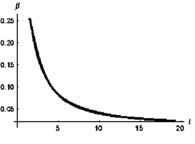
Fig. 4. Dynamics of the function p_M ( t ) for y 0 = 1, k = 12, g = 13, b = 2/3

will be occupied by specialists of the intermediate and low categories.

Denote p = lim p m ( t ) ,   y = lim у _M ( t ) ^.

t ^x             t ^X

Then p ₊ у = ^M - A , and, in addition, p

*

X ²

*

У 2

= z 2 ,

H ' m                 у hence, = z2(1 - AM), у = 1 - AIM .

1 + z 2            ^{1 +} z 2

Thus, the number of vacant jobs, which is being occupied in time by specialists of the intermediate and low categories, is divided into two set with known numbers of

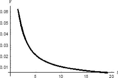
Fig. 5. Dynamics of the function y_M ( _t ) ^for y 0 = 1, k = 12, g = 13, b = 2/3

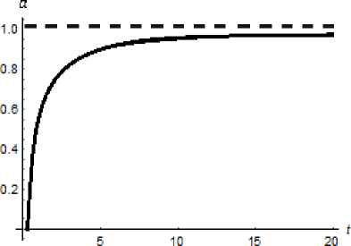
Fig. 6. Dynamics of the function _ам ( _t ) for y о = 1, k = 12, g = 13, b = 2/3

In the second case, we have A + B + G = M + N > A + N, hence A < M, that is the number of specialists of the high category in the labor market is less than the total number of workplaces. Note that a = lim aM (t) = А/M, therefore the enterprise t ^X can employ all specialists of the high category from the labor market. However, since A < M, still there will be vacant jobs, which elements by means of the constant z2 . Therefore, z2 is the ratio of the limit number of specialists of the intermediate category to that of specialists of the low category in the enterprise.

In Fig. 7, 8, 9 the graphs of the ^functions a M ( t ) , P M ( t ) , у M ( t ) ^are represented for the second case.

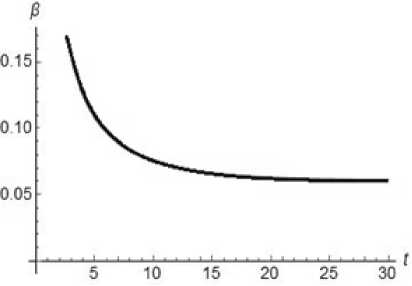
Fig. 7. Dynamics of the function p_M ( t ) ^for y о = 1, k = 12, g = 13, b = 12

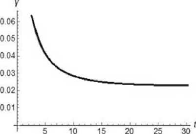
Fig. 8. Dynamics of the function у_м ( t ) for y о = 1, k = 12, g = 13, b = 12

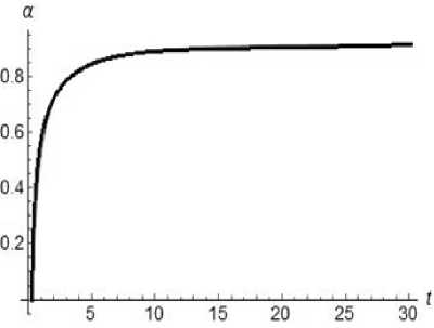
Fig. 9. Dynamics of the function _ам ( t ) for y о = 1, k = 1/2, g = 13, b = 12

1 1 b + g -1 ]  g   G   n у = lim у(k) = lim — I —-— I = — = — > 0.

k >+ 0       k >+ 0 m / 1 + Z ( k ) J   m  M

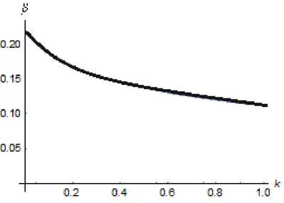
Fig. 10. Dynamics of the function p ( k ) for m = 3, g = 4/3, b = 12

Till now we have considered the

coefficient k to be a constant. Now we try to find out how one can influence the quantitative and qualitative structure of the set of the employed subjects by changing the coefficient k. This changing does not effect the value a = ^m a (t), however it effects the t >x values p = lim pM (t) and Y = lim уM (t), since t >Л                         t >OT they does not depend on z 2 and, hence, on k

. Thus, p = p ( k ) , у = y ( k ) .

Consider        the        function z 2 = Z( k) =

1 - k + kb - g + (1 - k + kb - g )² + 4 kgb

2 kg in the interval (0,1]. This function is continuously differentiable in (0,1], and also Z( k) < 0, hence z( k) monotonically decreases.

Its behavior in the neighborhood of zero is characterized by the following limit relation:

—, ff g > 1

lim Z ( k ) = ^ g - 1

k >+ 0

+OT   ff  g <  1.

By (14), the analysis of the situation, when there are vacant jobs in the enterprise after all specialists of high category are employed, requires considering two cases (Fig. 10, 11) defined by the sign of the number g - 1 = g/n - 1 .

Case A. Suppose G >  N . Pass to the limit as k >  0:

Z(k) /b+g -1 ^  ьв

P = lim P(k) = lim     I-------I = — = — k>+0      k>+0 m 1 1 + Z(k) j  mM

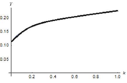
Fig. 11. Dynamics of the function у ( k ) for m = 3, g = 4/3, b = 12

So, in case А it is not possible to reduce the number of specialists of the low category to zero, even if the work with personnel is carried out with maximal intensity. The fraction of specialists of the low category in the enterprise cannot be less than the positive value GM . This part of the staff of the enterprise will be rotating permanently.

Case B. The more interesting is the case, when G <  N , that is the number of specialists of the low category is less than the total number of the unemployed. Here the coefficient k is playing a vital role.

For example, if k = 1 (the work with personnel is not carried out at all), we get z ₂ = Z (1) = b/g = B/G , that is the ratio of the number of specialists of the intermediate category to that of specialists of the low category in the enterprise is the same as the analogous ratio in the labor market in general.

Let us show (Fig. 12, 13) that the quality of the staff of the enterprise can be improved by diminishing the value of k.

Z(k) f b + g -1 / b + g -1 M - A в = lim P(k) = lim —I —-— I = —-— =----, k >+0      k>+0 m / 1 + Z(k))     m      M

Y* = lim y(k) = lim — ------- k>+0       k>+0 m ^ 1 + Z(k) ^

= 0.

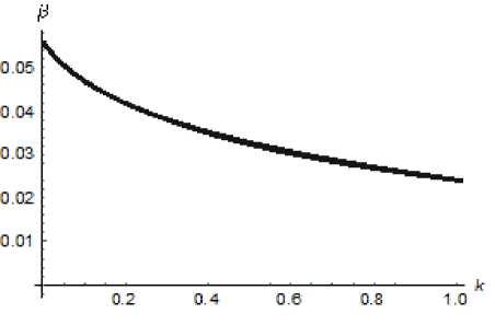
Fig. 12. Dynamics of the function p ( k ) for m = 3, g = 2/3, b = 1/2

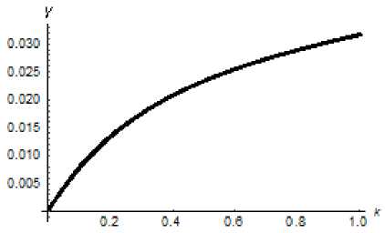
Fig. 13. Dynamics of the function y ( k ) for m = 3, g = 2/3, b = 1/2

From above, it follows that in case В one can theoretically reduce the number of specialists of the low category to zero by directing k to zero. In practice, this means that intensive work with specialists of the intermediate category gives the enterprise an opportunity to make the number of specialists of the low category negligible.

Speaking about the economic interpretation of the results we should say that in the research it was established that if the number of highly qualified specialists exceeds the number of jobs at the labor market, then the rational behavior of the employer guarantees 100% professionalism of the staff, and, as a result, the maximum efficiency of the functioning of the enterprise. However, first, not all employees of good qualifications will be able to find work; second, there is a problem associated with a staff turn-over due to the absence of motivation to increase qualification level. Unsatisfied labor supply can mean, for example, a high unemployment rate among citizens with higher education. The labor market with excess labor can be a consequence of the re-training of specialists in a given sphere or the low level of development of enterprises on which these specialists are in demand. This problem can be solved either by expanding the labor market and opening new vacancies, or by changing the course of staff training due to expanding budgetary places in universities, demand for whose graduates is higher, due to the reduction in the number of budget places in other universities.

If all highly qualified specialists have an opportunity to find a job, and still the unsuccessful demand for labor remains on the part of the employer, it is possible to improve the efficiency of the enterprise by improving work with personnel, thus bringing the labor market conditions closer to its equilibrium state. However, in the case of an excess of inadequate qualifications in the labor market, there will always be a number of vacancies in the enterprise, which characterizes the labordeficit market situation. In Russia, this phenomenon is observed, for example, in firms that distribute advertisements, as well as in real estate agencies, which are characterized by high staff turnover. This problem is solved either by a reduction in the number of staff members, or again by opening institutions engaged in the training of specialists whose work is in high demand.

Conclusion

In the present paper a new mathematical model of labor market conditions has  been proposed and described by means of a system of differential equations. The model is simple for understanding and presentation. However, it is meaningful, since a complete mathematical analysis of the system carried out in the work made it possible to reveal significant qualitative and quantitative characteristics that determine the dynamics of the labor market.

It is interesting to note that the model of a closed mono-branch labor market conditions considered above makes it possible to describe some other processes that are typical for different markets. For example, applicants applying for places in higher education (or undergraduate students) can also be divided into three conditional categories by analogy: first, subjects with a high level of training and abilities for this specialty; second, those who are potentially capable of learning; third, those, who are either not capable or have no will to learn. In this case the coefficient k can be interpreted as the level of rigor of the receiving commission (or that of qualifications of the teachers) of the given institution.