Modeling of an optimal trajectory at a safe distance in a spacecraft cluster

The cooperative movement of spacecraft, including rendezvous, undocking, and flyby maneuvers, is one of the most important challenges in modern space technology. The growing number of small spacecraft groupings and the development of space debris inspection, maintenance and removal missions increase the requirements for autonomous control methods that ensure the safety of relative movement with limited resources of the propulsion system and orientation system [1–4]. In this context, the construction and analysis of optimal control laws that guarantee movement at a given safe distance is of practical interest and at the same time remains a non-trivial task from the point of view of optimal control theory.

In this paper, the task involves modeling the optimal trajectory of a deputy satellite relative to a reference satellite during the undocking maneuver and subsequent flyby at a safe distance. A linearized model of dynamics based on the Hill – Clohessy – Wiltshire equations [5; 6] written in an orbital coordinate system is used to describe relative motion. The quality of control is assessed using an integral functional that characterizes the tendency of the position of the deputy spacecraft to the limit of the permissible range. The choice of functional capabilities thus allows for maintaining movement at a safe distance and reflecting the physical meaning of the maneuver under consideration.

An analysis of the problem formulation reveals that the problem is highly complex, both analytically and numerically, due to the structure of the functional and the presence of phase and control constraints. Therefore, a decomposition method is used in this paper, allowing the original problem to be divided into two subproblems: studying motion along a boundary trajectory and solving the time-optimal problem of ensuring the deputy satellite reaches the boundary of the feasible region. The re- sulting subproblems are analyzed using Pontryagin's maximum principle, along with numerical modeling and a comparative analysis of control strategies.

The first part of the paper presents a mathematical model of relative motion and the formulation of the original optimal control problem. Next, the decomposition of the original problem is considered, and the subproblems of reaching the boundary and motion along the boundary trajectory are analyzed. Then the results of numerical modeling for circular and elliptical trajectories are presented.

Mathematical model and problem statement.

The O xyz orbital coordinate system associated with the reference satellite is used to simulate the relative motion of two spacecraft. The coordinate origin is aligned with the reference satellite's center of mass, the O x axis is directed along its radius vector, the O z axis is normal to the orbital plane in the direction of the orbital angular momentum, and the O y axis completes the system to form a right-hand triad. This system considers the motion of the deputy satellite relative to the reference satellite.

The initial model is the equation of motion for each spacecraft in an inertial coordinate system in the Earth's central Newtonian gravitational field. The radius vector r satisfies the equation:

r

r = -Ц—т, r3

• •

where μ is the Earth's gravitational parameter. The relative position vector of the deputy satellite is defined as p = r p - r t , where the indices p and t refer to the deputy and reference satellites, respectively. The transition to an orbital coordinate system leads to equations of relative motion in a non-inertial system, which take into account the Coriolis and centrifugal terms.

To obtain the linear model used in this paper, standard assumptions used in close-rise and flyby problems are introduced:

• 1)    the orbit of the reference satellite is considered circular (with a constant average motion of n );

• 2)    the motion occurs only in the central field with a Newtonian potential, and perturbations are ignored;

• 3)    the relative distance between the satellites is small compared to the radius of the reference satellite's orbit, so the small parameter is the ratio r / r c , and higher-order quantities are discarded.

When these assumptions are met and linearized in small relative coordinates, we obtain the Hill– Clohessy–Wiltshire (HCW) system for relative motion in the orbital coordinate system [7]. This paper considers the planar case, when the motion occurs in the orbital plane O xy , and the z coordinate and the corresponding equation are not used. The linearized system has the form

• x = 3 n ² x + 2 ny + F_x , y = - 2 nX + F_y .

  
  

Here x(t) and y(t) are the relative coordinates of the deputy satellite in the orbital coordinate system; n is the average motion of the reference satellite; F x ( t ) and F y ( t ) are the control forces generated by the deputy satellite's propulsion system and directed along the O x and O y axes. The choice of a linear HCW model allows us to preserve the main physical effects of relative motion in a near-circular orbit (the gravitational-inertial relationship between coordinates and velocities, the Coriolis terms 2 n͘y and 2 n͘x ), while obtaining a compact system convenient for formulating and analyzing optimal control problems.

Control is specified through the thrust magnitude f ( t ) and its direction angle φ( t ) in the O xy plane. Then the components of the control forces have the form

The thrust modulus is assumed to be bounded from above, 0 ≤ f ≤ f max . Furthermore, a constraint on the rate of change of thrust direction is taken into account: a control action is introduced: u ( t ) = ͘φ( t ), for which |u| ≤ u max . This choice of control parameterization corresponds to a situation where the engine provides a thrust modulus limited by its modulus, and the attitude control system (or thrust vector control system) has a limited rate of thrust direction rotation.

To bring the dynamics to the standard form of an optimal control problem, the state variables are introduced: x 1 = x , x 2 = ͘ x , y 1 = y , y 2 = ͘ y . Then the HCW system is written as

' *1 = x 2, x2 = 3 n2 x1 + 2 ny 2 + f cos ф,

• y , = y 2 ,                                                             (4)

y 2 =- 2 nx 2 + f Sin ф ,

ф = u.

The initial conditions correspond to the moment of undocking, when the deputy satellite coincides with the reference satellite in position and relative velocity: x 1 (0) = 0, x 2 (0) = 0, y 1 (0) = 0, y 2 (0) = 0. The value of φ(0) can be specified as the initial orientation of the thrust direction; it is then determined by the equation for ͘φ.

To ensure flight safety, an acceptable relative position region is introduced as a circle of radius r in the O xy plane. The study utilizes an integral performance criterion that reflects the system's tendency to approach the boundary of the acceptable region while maintaining the requirement to remain within it throughout the entire control interval. The functional is the integral of the margin to the boundary along the radial direction:

J = j 0 r ² - x ²( t ) - y ²( t ) dt ^ min.                             (5)

Problem decomposition method

The value of the integrand is non-negative within the feasible region and vanishes at the boundary of the safe zone. Therefore, minimizing the functional J corresponds to a regime in which the deputy satellite strives to reach the vicinity of the safe zone boundary as quickly as possible and then remain close to it for as long as possible without leaving the feasible region. Thus, the optimal control problem consists of choosing functions f ( t ) and u ( t ) on the time interval [0, Т ], that satisfy the constraints and ensure a minimum of the functional J while satisfying the equations of motion.

Direct implementation of the original formulation with an integral functional and phase constraint proves computationally complex, so a decomposition method is used and two sequentially solved subproblems are considered. The first stage involves reaching the boundary of the feasible region in minimal time, i.e. it is formulated as a time-optimal problem. The second stage involves moving along the boundary and maintaining the trajectory in its vicinity under given constraints on the control actions.

It's important to note that this decomposition reformulates the original problem: the resulting subproblems no longer preserve the phase constraint of the original problem. Therefore, trajectories found within the decomposition may generally extend beyond the safe zone, and this effect must be separately monitored and analyzed based on the simulation results. In this regard, the "smooth approach" strategy is of particular interest: a tangential approach to the boundary ensures a more consistent transition to the second stage and effectively helps maintain the phase constraint, reducing the need for subsequent correction.

Reaching the boundary

Consider the performance problem. The dynamics of the system and the control constraints remain the same as in the original problem, but instead of the integral functionality, the final time T is minimized. The absence of an integral function simplifies the application of the Pontryagin maximum principle and leads to a simpler structure of the Hamilton function [8–10]. For the performance problem, it has the form

H ( x , u , v ) = v x 1 x 2 + v x ₂ ( 2 ny 2 + 3 n ² x i + f cos ф ) + V y y 2 + V y ₂ ( - 2 nx 2 + f sin ф ) + ¥ ф u — 1. (6)

Here x = ( x 1 , x 2 , y 1 , y 2 , φ) is the vector of system variables; u is the control vector; ψ = (ψ x 1 , ψ y 1 , ψ x 2 , ψ y 2 , ψ φ ) is the vector of adjoint variables. For the speed-response problem with the adopted normalization, H includes a constant term -1. For an optimal solution with a free finite time, the following condition must be satisfied:

H ( t ) = 0, t e [0, T ].

The deviation of H from zero in the numerical solution is further used as one of the performance criteria, characterizing the degree to which the necessary optimality conditions are met.

Let's consider the control laws. According to Pontryagin's maximum principle [11], optimal controls are chosen so as to maximize the Hamiltonian over admissible controls for a fixed state and fixed adjoint variables. The control of the angular velocity u has a relay structure:

u( t ) = ^u max Sign ( ф_ф ⁽ t ) ) ,

where Sign( x ) = 1 for x > 0, Sign( x ) = -1for x < 0, and for x = 0 any value from the interval [-1, 1] is allowed.

We introduce the switching function S f ( t ) = ψ x 2 ( t )cos φ( t ) + ψ y2 ( t ) sin φ( t ). Then the optimal control with respect to f has the form

л f (t)=

S f ( t ) >  0,

S f ( t ) <  0,

and in the case of S f ( t ) = 0, the control can take any value from the interval [0, f max ], which corresponds to a special mode when executing S f ( t ) ≡ 0 on the time interval.

Movement along the boundary

In the second stage, after reaching the target trajectory, the task is reduced to maintaining it. To describe the position on the circle, we introduce the parameter θ( t ):

x 1 ( t ) = r cos 0 ( t ),      y 1 ( t ) = r sin 0 ( t ).                                (10)

Then the required control law, ensuring trajectory maintenance, can be written as f (t) = 3 n2 r |cos 0( t )|,

I П

^{ф (} t ) -k

cos 0 ( t ) >  0, cos 0 ( t ) <  0.

Here, φ is the thrust direction angle, and f is the magnitude of the control acceleration required to maintain motion along the boundary.

Angle switches near the upper and lower points of the circle θ = π/2 и θ = 3π/2 are permissible, since at these points cosθ ≈ 0, meaning the required thrust f ( t ) is practically switched off. Let's estimate the impact of the turn on the system dynamics. Assume the turn through angle π is performed with maximum angular velocity; then the switching time

Д T switch

П

u max

The switching interval θ( t ) passes through the neighborhood [π/2 – ε, π/2 + ε], where cosθ < ε, therefore the average value of the thrust can be estimated as

7 2 2 ⁶

f « 3 nr— . 2

The change in angular velocity of movement on such a short section can be estimated as

ле . f- . 3^5

.

ru u max max

Since θ ' is of order 2 n near the boundary, ε ≈ |2 n |Δ T switch /2 = | n |π/ u max , and then

A0«

3 n | n |³

^{2 u} max

For the numerical experiments, the following values were used: n = 0,0011 rad/sec and u max = 0.2 rad/sec. We obtain Δθ' ~ 10^–7 rad/sec, which is negligible compared to |͘θ'| ~ 10^–3 rad/sec. Consequently, the engine rotation near the upper/lower point of the circle can be considered practically instantaneous and does not lead to a noticeable deviation from the trajectory.

Numerical modeling of the trajectory

Calculations were performed for two types of target trajectories: circular and elliptical, defined by the periapsis and apoapsis parameters ( r p , r a ). In both cases, a two-stage scheme was used, consistent with the adopted problem decomposition. The first stage solved the boundary approach problem (in a time-optimized formulation) taking into account control constraints, and the second stage completed the construction of the full trajectory by simulating motion along the boundary and maintaining it there. Two approaches were used to solve the first stage: an indirect method (shooting method), based on Pontryagin's maximum principle and reduction to a boundary value problem, and a direct method implemented in the CasADi library [12], which reduces the problem to nonlinear optimization after time discretization. The full trajectory was completed by integrating the original ODE system under a closed control law for motion along the boundary and taking into account constraints on the thrust and the rate of rotation of the thrust direction.

For the numerical implementation, the model constants and parameters n, T, umax, fmax, were fixed, determining both the scale of the dynamics and the achievable class of trajectories under given control constraints. The mean motion n was chosen based on the parameters of the reference circular orbit and calculated using the formula n = ^3, Ц = 3,986 x1014m3/sec2, (16)

where μ is the Earth's gravitational parameter; R is the radius of the reference orbit. An orbit at an altitude of 500 km above the Earth's surface was considered:

R = R E + 500 m = 6,371 x 10 6 + 5 x 10⁵ = 6,871 x 10 6 m,                 (17)

where from we get the estimate

n

3,986 x 10¹⁴ (6,871 x 10⁶)³

» 0,0011 rad/sec.

The limit on the angular velocity of the thrust direction change is set via the control u = φ' rad/sec. For small motor systems, typical values are of the order ± 10° = 0.17 rad, therefore, the calculations took u   = 0, 2rad/sec.

max

The acceleration module limit was chosen in the range typical for small spacecraft. The base value was f   = 0,01 m/sec2 .

max

Circular trajectory

Numerical calculations for the circular trajectory at the first stage were performed using the shooting method – a numerical algorithm for solving boundary value problems for systems of ordinary differential equations [13–15]. The system being solved included the Hill–Clohessy–Wiltshire equations and equations for adjoint variables derived from a system of necessary conditions. This yielded extremals – trajectories satisfying the necessary optimality conditions and serving as candidates for the optimal solution. Two control options were considered: 1) control using the Pontryagin method (this approach involves using a control law derived from the Pontryagin maximum); 2) control with maximum thrust (in this case, the thrust is always maintained at its maximum). Smoothed control laws were used in the numerical implementation of both approaches, which increased the stability of the integration and improved the convergence of the algorithms. The calculations were performed for target circle radii r = 50, 100, 500, and 1000 m. All graphs are presented for the case of r = 100 m. The phase trajectories for the first stage are presented below (Fig. 1).

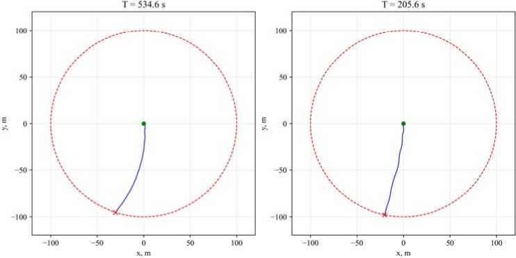
Рис. 1. Управление по методу Понтрягина (слева) и управление с постоянной тягой (справа)

Fig. 1. Control obtained by Pontryagin’s method (left) and control with constant thrust (right)

In addition to the shooting method, based on the analysis of a system of necessary conditions and Pontryagin's maximum principle, optimization methods were used, in which the optimal control problem, after time discretization, is reduced to a nonlinear programming problem. The CasADi library was used to implement the direct approach.

A trajectory using the "smooth approach" strategy was also constructed using direct methods. This variant additionally specifies a condition on the final state: the relative velocity vector must be tangent to the target circle. This requirement typically increases the time to reach the boundary at the first stage and, as a result, can lead to an increase in the value of the initial functional. However, at the second stage – when moving along the target trajectory – a near-zero value of the functional is expected, since the need for significant trajectory correction becomes minimal. The corresponding trajectories obtained in CasADi are shown in Fig. 2.

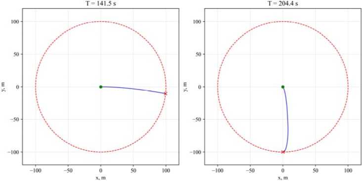
Рис. 2. Траектория, полученная с использованием CasADi: стандартная траектория (слева) и гладкий подлет (справа)

• Fig. 2.    Trajectory obtained using CasADi: standard trajectory (left) and smooth approach (right )

The geometric meaning of the initial functional is related to the distance of the trajectory from the target circle. To compare numerical algorithms and control strategies, a graph was constructed of the dependence of the distance to the target circle on time (Fig. 3).

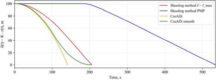
Рис. 3. Зависимость расстояния до целевой окружности от времени

• Fig. 3.    Distance to the target circle as a function of time

It can be seen that the longest time to reach the boundary is demonstrated by the firing method with a control law derived from Pontryagin's maximum principle: for R = 100 m, the obtained value is T = 525.28 sec. During the initial portion of the trajectory, the distance to the boundary of the safe zone remains virtually unchanged, meaning the vehicle remains near its initial state for a long time. This is explained by the fact that the initial point (zero relative coordinates and velocities) is the equilibrium of the uncontrolled Hill-Clohessy-Wiltsher system: for f ( t ) = 0 and the same initial conditions, the solution remains identically at this point. Therefore, to exit the equilibrium, the thrust must be engaged.

Fig. 4 shows the control curves obtained using the shooting method. It is clear that the thrust modulus remains zero for a significant period of time, and it is this "lag" in thrust that is the key reason for the significant lag between the pure shooting method and the other approaches in terms of time to reach the limit.

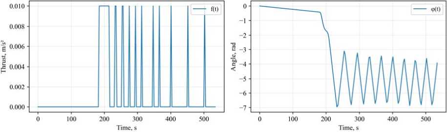
Рис. 4. Управления, полученные методом стрельбы (ПМП) на первом этапе при R=100 м

Fig. 4. Controls obtained by the shooting method (PMP) at the first stage for R = 100 m

If an extended section with near-zero thrust emerges along the determined extremum, the time to reach the circle increases significantly. It was this feature, combined with the indirect method's sensitivity to the choice of initial adjoint variables, that motivated the consideration of an alternative strategy with constantly active thrust. For this strategy, the time to reach the boundary was T = 210.00 seconds, i.e. approximately 2.5 times shorter than the Pontryagin shooting solution.

Let's now consider the solutions obtained using direct optimization methods in CasADi. At the start of the motion, both problem statements – the baseline and the "smooth approach" strategy – demonstrate similar dynamics and comparable gap reduction rates. However, in the final section, the trajectory with the "smooth approach" strategy approaches the circle more smoothly: the additional final condition (the tangent direction of the velocity vector to the target trajectory) reduces the need for subsequent correction in the second stage. As expected, this leads to an increase in time in the first stage (for R = 100 m: T = 204.38 sec versus T = 141.50 sec for the baseline formulation). However, the increase in time is moderate and can be offset by the gain in the second stage when moving along the boundary (due to smaller corrections, for example, by the PD controller).

For comparison with the direct optimization scenario, we present the controls found in CasADi for the baseline setup and for the "smooth approach" variant (Fig. 5). In both cases, the thrust is almost fully engaged, confirming our previous experiment, which demonstrated that using constant thrust control can be an effective method for minimizing the time to reach the boundary.

The control graph also shows that unlike the shooting method, in which the engine rotates at maximum speed, the CasADi solution does not exhibit such abrupt changes. This is confirmed by the smoother engine rotation, where its direction changes gradually, without sudden jumps. This is especially noticeable in the first case, where the thrust direction changes smoothly over time. This behavior is due to the fact that the adjoint variable for the thrust direction angle is set to zero during the optimization process, a special case that avoids excessive angular jumps and minimizes thrust switching.

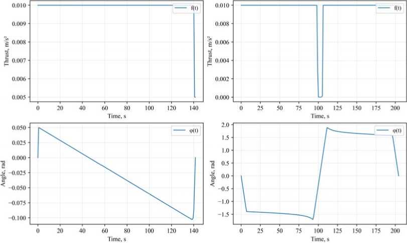
Рис. 5. Управления, полученные в CasADi на первом этапе при R = 100 м: базовая постановка (слева) и стратегия «гладкого подлёта» (справа)

Fig. 5. Controls obtained in CasADi at the first stage for R = 100 m: baseline formulation (left) and the “smooth approach” strategy (right)

Let's look at the numerical simulation results for target circles of various radii. Table 1 presents the key metrics of the first stage (boundary approach) for various methods: the time T required to reach the boundary, as well as the standard deviation of the Hamiltonian from zero.

Table 1 shows that the best boundary approach time for all radii is achieved by the direct CasADi implementation without additional final conditions, while the "smooth approach" option predictably yields slightly longer times due to its more stringent final state requirements. The strategy with constantly on thrust demonstrates time values of similar order of magnitude and, importantly, confirms the practical feasibility of the "maximum thrust" mode as a working heuristic for breaking the HCW equilibrium and accelerating boundary approach.

Table 1

Results of the first stage for a circular trajectory

Method / R	50 m	100 m	500 m	1000 m
Shooting	T = 356.92	T = 525.28	T = 9698.04	T = 9698.81
(PMP)	H RMS = 5.9794	H RMS = 4.1913	H RMS = 3476.23	H RMS = 4783.64
Shooting,	T = 148.83	T = 210.00	T = 432.14	T = 622.22
f = f max	H RMS = 0.0881	H RMS = 0.1873	H RMS = 1.3094	H RMS = 6.0624
CasADi	T = 100.15 H RMS = 0.3969	T = 141.50 H RMS = 0.7804	T=313.95 H RMS = 3.2968	T=439.91 H RMS = 6.2182
CasADi (smooth	T = 146.60	T = 204.38	T = 445.15,	T = 619.95
approach)	H RMS = 1.4979	H RMS = 2.7228	H RMS = 15.3737	H RMS = 37.2526

The solution obtained using the shooting method with Pontryagin's control law, on the other hand, results in a significantly longer time (and, for larger radii, a degradation of the result), which is consistent with the observed extended low-thrust region and the high sensitivity of the solution to the choice of the initial adjoint variables. It should also be noted that the deviation of the Hamiltonian from zero is significantly greater for this method, further confirming the assumption that for the problem under consideration, the optimal control structure tends toward a regime with constantly on thrust.

To interpret the results, it's important to consider not only the time it takes to reach the boundary, but also the state of the system as it approaches the target circle. Therefore, we will now examine the complete trajectories obtained using optimization methods and compare the baseline and the "smooth approach" strategy. Figure 6 shows a comparison of the phase trajectories in the ( x , y ) plane, allowing one to clearly assess the nature of the approach to the circle and the subsequent consistency of motion.

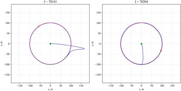
Рис. 6. Полные фазовые траектории: стандартная (слева) и гладкий подлет (справа)

Fig. 6. Full phase trajectories: standard trajectory (left) and smooth approach (right)

It is clear that the "smooth approach" strategy provides a more consistent entry onto the target circle: by the time the boundary is reached, the velocity vector is close to the tangent direction, so the transition to movement along the boundary can be accomplished with minimal corrective action in the second stage.

In the basic setup, the system strives to reach the boundary as quickly as possible, resulting in a relatively high absolute velocity and a noticeable radial component by the time the circle is crossed. This necessitates an additional "correction loop" near the boundary to absorb the excess velocity and align the motion with the boundary trajectory. This correction increases the overall costs of the original functional and complicates subsequent boundary containment.

Now let's look at the results obtained for various target circle radii: they are presented in Table 2.

Table 2

Results for different optimization methods

Method / R	50 m	100 m	500 m	1000 m
Shooting (PMP)	J = 15198.2544 HRMS = 697	J = 45281.1644 H RMS = 154	J = 4161573.7114 HRMS = 5506	J = 8226877.3510 H RMS = 7414
Shooting, f = f max	J = 6290.8716 HRMS = 288	J = 17711.1851 HRMS = 238	J = 185971.3978 HRMS = 618	J = 532970.5497 HRMS = 767
CasADi	J = 4378.4183 HRMS = 2701	J = 12373.7783 HRMS = 3803	J = 137460.6899 HRMS = 8231	J = 385843.4616 H RMS = 11130
CasADi (smooth approach)	J = 5251.7095 HRMS = 467	J = 14701.8696 HRMS = 615	J = 161547.3657 H RMS = 1792	J = 452666.5802 HRMS = 2965

A comparison of the results for the full trajectory confirms the conclusions of the first stage. Direct implementation in CasADi ensures stable trajectory generation for all radii and, as a rule, yields lower values of the functional J compared to the indirect shooting method, especially for large R , where sensitivity to the selection of initial conjugate variables and the presence of extended sections with low thrust lead to a noticeable increase in J . Moreover, the heuristic f = f max significantly improves the shooting result and approaches the order of magnitude of direct methods, which is consistent with the observed structure of the optimal solution: at the exit to the boundary, the thrust is often close to the maximum.

The "smooth approach" strategy naturally increases the time and J at the first stage due to the strengthened final conditions, but it ensures a more consistent entry to the boundary and reduces the need for subsequent correction at the second stage. Importantly, this strategy preserves the phase constraint contained in the original functional, meaning we remain within the safe zone at all times, a significant advantage over other methods. Next, we will consider the results for an elliptical boundary trajectory and compare them with the circular case.

Elliptical Trajectory

Now let's consider the case of an elliptical trajectory defined by the parameters of the pericenter and apocenter. Compared to a circle, an elliptical boundary has variable curvature and non-uniform thrust requirements along the trajectory, which can lead to changes in the control structure and different sensitivity of numerical methods. Below are the simulation results for an elliptical boundary and their comparison with the circular case. For clarity, the figures show an example for an orbit with parameters (100, 500).

Let's consider the full phase trajectories ( x, y ) obtained using direct optimization methods and compare the baseline case and the "smooth approach" strategy (Fig. 7).

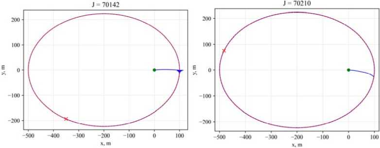
Рис. 7. Фазовые траектории для r a = 100, r p = 500: стандартная (слева) и гладкий подлет (справа)

Fig. 7. Phase trajectories for r a = 100 and r p = 500: standard trajectory (left) and smooth approach (right)

It's worth noting that, unlike the circular case, the stabilization of motion relative to the elliptical target boundary occurs differently. While for the circular case, stabilization was primarily provided by the "corrective loop," in this case, a mode of damped oscillations around the target curve is observed: the deputy vehicle periodically intersects the vicinity of the boundary, and the amplitude of the deviations decreases as it moves. This behavior is due to the variable curvature of the ellipse and the nonuniformity of the required holding thrust, as a result, the correction is distributed along the trajectory and manifests itself not as a separate maneuver, but as a gradual "muffling" of lateral deviations until stable tracking along the boundary.

To quantitatively assess the quality of the approximation, we next consider the "gap" to the elliptical boundary. The Δ r ( t ) graph (fig. 8) allows us to compare the velocity at the boundary in the first stage and the behavior of the trajectory near the target curve. As in the circular case, in the "smooth approach" variant, the completion of the approach occurs more smoothly: the gap approaches zero without sharp inflections, which is consistent with the additional final condition on the tangential direction of the velocity and reduces the need for correction in the second stage.

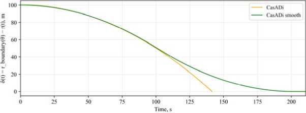
Рис. 8. Зависимость расстояния до целевой траектории от времени

Fig. 8. Distance to the target trajectory as a function of time

Figure 9 shows the controls obtained in CasADi: the thrust magnitude f ( t ) and the direction angle φ( t ). In both cases, f ( t ) is close to its maximum most of the time, which is consistent with the conclusions on the circular boundary and confirms the practical feasibility of a high-thrust strategy during the boundary approach phase.

The results for the full trajectory with various orbital parameters are presented in Table 3. They show that for an elliptical boundary, the "smooth approach" strategy yields comparable values of the J functional to the baseline formulation, while improving the alignment of the entry to the boundary and thereby reducing the need for corrective actions during the elliptical phase of motion. The observation that the thrust is close to maximum during the approach phase also holds for the elliptical case, which is consistent with the conclusions for a circle. The increasing complexity of the boundary geometry (variable curvature and non-uniform containment requirements) is reflected in a change in the H RMS index, so when comparing methods, the key criterion remains the complex approach criterion: the entry shape to the boundary and the value of the J functional along the full trajectory.

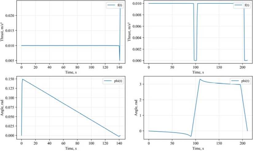
Рис. 9. Управления, полученные в CasADi на первом этапе для r a = 100, r p = 500: базовая постановка (слева) и стратегия «гладкого подлёта» (справа)

Fig. 9. Controls obtained in CasADi at the first stage for r a = 100 and r p = 500: baseline formulation (left) and the “smooth approach” strategy (right)

Table 3

Results for different optimization methods

Orbit parameters, m	CasADi (base)	CasADi (smooth approach)
(50, 100)	J = 93.69, H RMS = 8912.1104	J = 91.72, H RMS = 1668.7205
(50, 500)	J = 68.22, H RMS = 3198.9844	J = 52.68, H RMS = 3027.9954
(100, 500)	J = 113.47, H RMS = 4226.3390	J = 97.91, H RMS = 3775.8539
(100, 1000)	J = 108.02, H RMS = 6447.7756	J = 74.39, H RMS = 6736.8144
(500, 1000)	J = 342.02, H RMS = 9660.8593	J = 292.48, H RMS = 6474.9973
(500, 5000)	J = 353.17, H RMS = 14291.0808	J = 167.83, H RMS = 38524.5944

Conclusion

The study conducted for circular and elliptical target trajectories showed that in the given setting, direct optimization methods yield the most stable and reproducible solutions. The CasADi implementation allows for stable trajectories to be obtained for various parameters, phase constraints to be naturally taken into account, and additional final state requirements to be introduced without significant loss of computational stability. It is important, however, that the value of direct methods in this work lies not only in obtaining a numerical solution, but also in the fact that these solutions provide a basis for further analytical research: based on the structure of the obtained controls, the nature of constraint saturation, and the behavior of the trajectories, it is possible to identify typical modes and formulate hypotheses about the optimal control structure, which can then be tested using indirect methods.

A comparison of control modes during the boundary approach phase reveals that, in many cases, the numerically optimal solution utilizes thrust close to maximum for a significant portion of the interval, consistent with the physical meaning of the performance problem and indicating the dominance of the saturation mode with respect to fmax. Thus, the results of direct optimization help refine the ex- pected control structure and serve as a guide when constructing initial approximations and selecting parameterizations in indirect schemes. The indirect approach, on the other hand, proved to be significantly more sensitive to the choice of initial adjoint variables: in a number of modes, an extended low-thrust segment emerges, leading to a significant increase in the boundary approach time and, consequently, to a deterioration in the value of the initial functional. This indicates the need for further elaboration of the analytical conditions for the occurrence of such special segments, as well as the need to develop more robust initialization and continuation procedures for the shooting method.

The "smooth approach" strategy deserves special attention as it ensures tangential entry to the boundary. On the one hand, introducing additional terminal conditions naturally increases the costs in the first stage, as it narrows the set of feasible trajectories. On the other hand, numerical experiments show that the final value of the functional with this approach remains comparable to the baseline variant, and the transition to movement along the boundary trajectory is more consistent. This reduces the need for subsequent correction in the second stage and facilitates compliance with the phase constraint. However, the "smooth approach" strategy proves to be the most challenging for indirect methods due to the increased sensitivity of the boundary value problem and the complexity of the terminal conditions, highlighting the relevance of further research.

The results of this work should be viewed as a step toward constructing a more complete analytical picture of the two-stage maneuver "boundary entry + movement along the boundary." Direct optimization methods provide a reliable numerical base and allow us to identify characteristic control modes, while further development of indirect methods and analytical descriptions of the optimal solution structure requires taking into account the identified sensitivities, developing robust initialization schemes, and a more in-depth analysis of low-thrust regions. A combination of these approaches appears to be the most promising direction for further research.