Моделирование воздействия внутренних гравитационных волн на состояние верхней атмосферы в период внезапного стратосферного потепления

The internal gravity wave (IGW) is an important mechanism of interaction between processes in the lower and upper atmosphere. Propagation of IGWs from lower layers has a profound effect on many atmospheric and ionospheric phenomena [Pancheva, Mukhtarov, 2011]. An example of realization of such interactions is atmospheric disturbances that develop during sudden stratospheric warmings (SSWs)

SSW refers to a swift jump in temperatures in the stratosphere (up to 80° over the course of a few days) at high latitudes. The typical scale of a heated area can reach 4000 km in longitude. In winter, SSWs predominantly occur in the Northern Hemisphere [Harada, et al., 2010]. Today, there is a wealth of data on SSWs. At the same time, we have not yet had a full theoretical description of how SSWs appear and develop. The most popular hypothesis suggests an interaction between zonal mean flow and planetary waves in the stratosphere [Labitzke, Kunze, 2009].

An important feature of SSWs is their impact on atmospheric processes outside of a warming region. In particular, in [Pancheva, Mukhtarov, 2011; Polyakova et al., 2014; Shpynev et al., 2013] authors noted that SSWs have an effect on various ionospheric parameters such as the F2-layer critical frequency ( f o F2), its height maximum ( h _mF2), and total electron content (TEC). Of special interest are data on variations in ionospheric parameters at low latitudes, situated thousands of kilometers away from an SSW region [Sumod et al., 2012]. An analysis of long-term observations allows us to assume that the response of the upper atmosphere and ionosphere to SSWs is caused by intensification of tidal activity at heights of the lower thermosphere, which induces variations in electric fields in the ionospheric dynamo region and respective effects in the ionosphere. Results of simulation studies show in general that different schemes for intensification in tidal variations in the lower thermosphere during SSWs make it possible to qualitatively model spatial and temporal peculiarities of ionospheric disturbances; however, theoretical amplitude characteristics prove to be far less than observable ones.

Observations indicate that the time delay in the occurrence of disturbances in the lower atmosphere and ionosphere is quite insignificant as compared to the duration of SSW and periods of planetary waves. It is fair to assume that the physical mechanism ensuring fast interaction between the dynamics of the lower and upper atmosphere can be IGWs excited in an SSW region. Indeed, experimental investigations report observations suggesting that IGW activity increases during SSWs [Wang, Alexander, 2009]. Karpov, Kshevetskii in their theoretical study [Karpov, Kshevetskii, 2014] show high efficiency of such waves propagating from the lower atmosphere in the formation of large-scale disturbances in the upper atmosphere.

The purpose of our study is to explore the possibility of exciting IGWs, able to propagate to the upper atmosphere, by disturbances of stratospheric parameters during SSWs.

DESCRIPTION OF THE NUMERICAL EXPERIMENT

We perform a numerical experiment, using a 2D non-hydrostatic model of neutral atmosphere that is based on the solution of non-stationary hydrodynamic equations for wave disturbances with respect to nonlinear and dissipative processes during wave propagation as well as their interaction [Kshevetskii, 2001]:

dp + d ( p u ) + d ( p w ) = о

dt    6x      dz      ’

d ( p u ) d ( p u 2 ) d ( p uw ) _ d t       6 x        d z d p d L, xuu ) =+    ^ ( z )     +^ ( z d x d z C d z J v d ( p w ) d ( p uw ) d ( p w 2 ) ——^ + _^--£ + _^ ^ = d t        d x        d z d P      5L, xww ) =P g +    ^ ( z ) d z       d z (     d z J 1 fd P d Pu d Pw ) +---+        = - Y - 1 ( d t d x     d z ) , . d2 T + K ( z )      + Q vis cos + Q ( z ): d x

x d2 u )d x 2 ’ d 2 w + ^ ( z ) ^T, d x - P V v + — K ( z d z (

Q(z) = -- K(z) ^ ( ) dz ( ) dz where x, z are the horizontal and vertical coordinates; ρ is the density; u and w are the horizontal and vertical components of velocity vector; P is the pressure; g is the free fall acceleration; γ is the adiabatic exponent; ξ(z), K(z) are the coefficients of viscosity and heat conductivity; T0(z) is the vertical temperature distribution in the initial condition; Q(z) is the parameter accounting for the additional heat inflow ensuring stationarity of the non-isothermal atmosphere under undisturbed conditions; Qρ is the source of density disturbance.

The equations for atmospheric parameters were numerically solved in a region of horizontal size 2000 km and vertical size 500 km from Earth’s surface.

For simulated parameters on the lower boundary we specify the following conditions:

u ( x , z =0, t )= w ( x , z =0, t )=0,

T ( x , z =0, t )= T 0 ( z =0),

ρ(x, z=0, t)=ρ0(z), where ρ0(z) is the vertical density distribution in the initial condition preset in the same manner as T0(z), using an empirical model [Picone et al, 2002]. On the upper boundary (h=500 km), we assume the following conditions

8 T     d u

— = 0; — = 0; w = 0; z = h .

d z      8 z

On horizontal boundaries of the integration domain ( x =0, 2000 km), derivatives of the simulated parameters in the coordinate x are equal to zero.

As a source of disturbance we specify a temperature and density disturbance according to observed data on the January 2009 warming. During development of this SSW that occurred under low solar activity and quiet geomagnetic conditions, a large amount of experimental research was done into variations of atmospheric and ionospheric parameters. Specifically, there are lidar sounding data that allow us to reconstruct the temperature profile over the SSW and its difference from the undisturbed one [Kurkin et al., 2011; Shpynev et al., 2013]. Based on these data, data on temporal variability of temperature at various heights [Jin et al., 2012], and the IGW propagation theory [Grigoriev, 1999], a model of temperature disturbances in the stratosphere during SSWs has been developed.

The analysis of stratospheric observations [Shpynev et al., 2013] has revealed two time-dependent components in temperature variations – a long-period one with a period of 20 days and an amplitude of 80 K and a short-period one with an amplitude of 7 K and a period of 30 min, which are located at z ~35 km in a region with a vertical scale of 10 km.

In the numerical experiment, the simulated source is localized in a horizontal direction x . The disturbance amplitude is maximum at x = 0 and decreases with distance away from the left boundary of the model area. This choice of source location is in line with the modeling of the latitude structure of the southern half of the warming region. According to the IGW theory, polarization relationships for large-sale waves having a frequency that is much lower than the Brunt-Väisälä frequency allow us to identify an IGW-related density disturbance:

A T _ Ap T " P

where ∆ T and ∆ρ are respective temperature and density disturbances, T and ρ are their background values.

Thus, the disturbance source in (1) is described by the following expressions:

I x I

A T _ exp I - 2 lx

I x, )

x x exp p dAT

T dt , where A1=80, A2=7, xs=500 km, z0=35 km, zs=7 km, T1=20 days, T2=30 min, Tz=10 km.

Equation (3) shows that the amplitude of the source falls rapidly in a horizontal direction, and at 800 km it makes up several percent of its maximum. By convention this region is the horizontal boundary of the source.

At the beginning of numerical calculations, dynamic parameters correspond to the undisturbed atmospheric conditions specified by the empirical model [Picone et al., 2002]. The disturbance source has been working continuously for 12 hr during the numerical experiment.

The modeled source of stratospheric disturbances determines frequency of variations in atmospheric parameters in the localized region. The spatial and temporal structure of disturbances will be defined by a wide range of waves excited by this oscillation process in an inhomogeneous atmosphere as well as by their interaction as they propagate to the upper atmosphere. Amplitude disturbances of stratospheric source parameters, which are governed by long-period and short-period processes in a time interval equal to the duration of numerical experiment, are comparable.

EXPERIMENTAL RESULTS

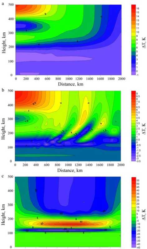
Figure 1 illustrates spatial distributions of temperature disturbances relative to initial atmospheric conditions at different moments of time after the start of the numerical experiment. At the initial stage of calculations, for the first hour of the modeling, a transient process took place which consisted in heating the region directly over the source nearby the left boundary of the simulated space (Figure 1, a ). Within 2.5 hr after the start of the calculation at heights over 100 km, a wave process occurs that involves expanding the region of disturbances in a horizontal direction and forming a region with maximum disturbances over the horizontal boundary of the stratospheric source.

О 200   400   600   800  1000 1200 1400 1600 1800 2000

Distance, km

Figure 1. Distribution of temperature disturbances in 1 ( а ), 2.5 ( b ), and 10 hr ( c ) after the start of the calculation

As the calculation continues, the disturbance amplitude increases in a height interval 100–200 km, and the disturbance maximum shifts toward the horizontal boundary of the source. After 10 hr of calculations, the disturbance amplitude reaches 50 K (Figure 1, c ). Figure 2 pictures spatial temperature distributions in the upper atmosphere for two moments of time after the start of the numerical experiment. It is apparent that the developing wave process is reflected in temperature variations in the upper atmosphere. Maximum amplitude disturbances of the background temperature are ~40–60 K. They occur above the horizontal boundary of the source (Figure 2); their period is ~3 hr.

Thus, the results of the numerical experiment show that temperature and density disturbances arising at stratospheric heights during SSWs propagate rapidly, over the course of a few hours, to heights of the upper atmosphere and alter conditions in the medium. Maximum relative temperature disturbances with respect to undisturbed conditions are most pronounced between 100 and 200 km above the horizontal boundary of the source. As inferred from the results of the calculations, periods of disturbances in the upper atmosphere differ from periods of oscillations generated by the stratospheric source. This is due to the fact that the oscillation process in the stratosphere excites a wide range of wave disturbances, depending on frequency of forced oscillations and spatial sizes of the source, as well as on nonlinear and dissipative processes accompanying wave propagation to the upper atmosphere.

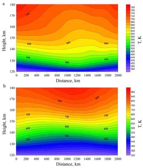
Figure 2. Background-temperature distribution within 10 ( a ) and 12 hr ( b ) after the start of the calculation

It is evident that such disturbances in the upper atmosphere affect in turn the dynamics of charged component in the ionosphere. The proposed mechanism of disturbances in the upper atmosphere works independently from disturbances of tidal variations which are generally considered in the modelling of ionospheric effects of SSWs. Accordingly, ionospheric disturbances initiated by IGWs from stratospheric sources can be treated as an additional contribution to observable ionospheric effects of SSWs. Notice that we conducted the numerical experiment using the 2D model, and therefore its results cannot fully reveal the dynamics of real atmosphere since the lifetime of a large-scale irregularity necessitates taking into account the effect of Coriolis force, i.e. three-dimensional consideration. At the same time, the effect of the stratospheric IGW source on conditions and wave activity in the upper atmosphere is demonstrated by observations and is confirmed by results of the numerical simulation.

The work was supported by the grant from the Ministry of Education and Science of the Russian Federation No. 3.1127.2014/K and the RFBR grant No. 15-05-01665.