Numerical algorithm and computational experiments for one linear stochastic Hoff model

Theoretical and applied research associated with the tasks of information processing and analysis, identification and management uses stochastic models [1–3] to assess the state and parameters of complex physical and financial systems. Of note, Sobolev type stochastic equations (1) have been used for several decades to describe and simulate a large number of physical, technical and technological processes

LdZ = MZdt + NdW.                        (1)

Analytical and numerical investigations of non-classical stochastic models are developing in two directions. One of them uses the concept of “white noise” as the Nelson– Gliklikh derivative of the Wiener K -process [4, 5]. This approach has been widely used in recent years for Sobolev type stochastic equations in the works of G.A. Sviridyuk, A. Favini, A.A. Zamyshlyaeva, S.A. Zagrebina, N.A. Manakova, M.A. Sagadeeva, T.G. Sukacheva [6–10] and for Leontief type stochastic systems in the works of Yu.E. Gliklikh, E.Yu. Mashkov [5], G.A. Sviridyuk, A.L. Shestakov, A.A. Zamyshlyaeva, A.V. Keller [11].

The other direction relates to development of the Ito–Stratonovich–Skorokhod approach [5]. It is one of the very first areas of investigation of differential equations and is currently considered classical. In the works of G. Da Prato, J. Zabczyk [12] the Ito– Stratonovich–Skorokhod approach is applied in the infinite-dimensional case. The works of I.V. Melnikova [13] investigate stochastic equations in Schwarz spaces, while using the traditional approach to the concept of white noise as a generalized derivative of the

Wiener process. M. Kov a cs and S. Larsson [14] investigated non-degenerate models of mathematical physics using the Ito–Stratonovich–Skorokhod approach. In the last decade, the works of G.A. Sviridyuk, A.A. Zamyshlyaeva [15], S.A. Zagrebina [16] investigate non-classical stochastic models within this approach. Therefore, new results for the theory of Sobolev type stochastic equations enabling the investigation of various mathematical models with the development of numerical methods and algorithms are relevant.

Suppose that G = G ( V ; E ) is a geometric graph, V = { V i } denotes a set of vertices and E = { E j } denotes a set of edges. On the edges E j of the graph G let us consider the linear stochastic Hoff equations

Ad j + du jxx = e j Z j dt + NdW j (2) with an initial–final condition

P o ( Z ( to ) - ( o ) = P 1 (Z ( ti ) - 6) = 0 , (3)

where W = (W 1 , W ₂ ,..., W n ) is an F -digit nuclear K -Wiener process, operator K E C (Z) is nuclear, P ₀ ,P 1 are relatively spectral projectors. At the vertices Vi of the graph G let us set continuity conditions

Z j (0,t) = Z k (0 ,t ) = Z m (l m ,t) = Z n (l n ,t), E j ,E k E E ^a (V),E m ,E n E E “ (V i )

and flow balance conditions

£ d j z jx (0,t) - £ d k Z kx (i k ,t ) = 0 , E j E E ^a ( V ) E k E E “ (V i )

where E ^a (V i ) (E ^ш ( V i )) is the set of edges having, at the vertices V i which is the beginning (end), l j >  0 and d j >  0 which are the length of the edge and the diameter of its cross section. Equations (2) describe the buckling dynamics of I-beams in a structure under constant load with a random external action. Here, the A E R ₊ parameter characterizes the load on the j th beam, the в E R parameter, in turn, describes the properties of the j th beam material, the random Z j = Z j (x,t), (x,t) E (0,l j ) x R process characterizes the deviation of the j th beam from the equilibrium position.

Let us turn to linear mathematical Hoff model [17]. Initial boundary value problems for the Hoff equation in a bounded domain Q were first studied by N.A. Sidorov [18] and his students [19, 20]. Hoff equations on a geometrical graph with the Cauchy condition were first studied by G.A. Sviridyuk together with V.V. Shemetova [21]. They managed to describe completely the phase space on a geometrical graph. Later, the inverse problem for the Hoff equation was solved on geometric graphs [22]. Furthermore, solution stability for the Cauchy problem of the Hoff equations was investigated, and sufficient conditions for stability and asymptotic stability of solutions to the Cauchy problem for the Hoff equations in the domain and on a geometric graph were obtained [23]. Optimal control of solutions to the Hoff equation was studied by N.A. Manakova and her students (see, for example, [24]). Numerical investigation of the non-autonomous Hoff equation on a geometric graph with the Showalter–Sidorov condition was carried out in [25].

The linear stochastic Hoff model for deformation in an I-beam structure with a multipoint initial-final condition was analytically studied in [26] in the sense of Nelson– Gliklich derivative to the “white noise” concept, and in [27] in the sense of the traditional approach. [27] proves the solvability of the initial-final problem (3) for an abstract linear stochastic Sobolev type equation (2).

• Theorem 1. Suppose the process W is the F ¹ -digit K -Wiener process, the operator N E L ( F 1 ) and for each fixed t random variables « ₀ ,« 1 E L 2 (Q , Z 1 ) and the W process are independent. Then for any « ₀ ,« 1 E L 2 (Q , Z ¹ ) the problem (2), (3) has a unique solution defined by expression

Z(t) = Z^ « 0 + [ %-L^Q o NW(s)ds +

^τ0                                                            (6)

+ Z t ^{- T1} « 1 + У Z 1 ~^g L - Q 1 NW (s)ds,

τ 1

where Z ₀ и Z ₁

— As I - S 1 ) ^{- 1} e ^s1 ds. 2пг J

γ 1

Z 0 =

2^ J(s I - S o ) -¹ e“ ds, Z 1 = γ 0

1.    The Algorithm of the Numerical Method

We will look for an approximate solution of the problem (2) – (5) in the form of

^Z (x,*) = [^Z 1 ^{( x} ₎ ^{t )} >^Z 2 ^{( x},^{t )} ,-,^Z n ^{( x},^t)j ,                               ⁽⁷⁾

where Z j (x,t) is the approximate solution on the j th beam of the graph of the form

N

0 ⁽ x, t ) = C N ⁽ x, t ) = £ a k ⁽t№ ^{( x )} .                         ⁽⁸⁾

k =1

Here, {^ k } = {^ k , ^ k ,...,^ N } refer to the corresponding orthonormal eigenfunctions relative to the scalar product of L 2 (G) .

Next, we apply the representation (8) to the Hoff equation (2), resulting in a system of equations by scalarly multiplying by eigenfunctions. Each system’s equation will contain only one unknown Galerkin coefficient; therefore, the expression (8) is a partial sum of the series, whose convergence provides for the convergence of the approximate solution to the exact one.

Note that the linearized Hoff model is considered on the graph. Let us build a description of the algorithm of the numerical solution.

Step 1. Given: N is the number of summands of the Galerkin sum; l j , d j are the length and cross-sectional area of the edges of the graph, respectively (equal for all edges), ω is the parameter of external action, a random variable A . λ j , β j are the coefficients of the linear Hoff equation. The coefficients are taken equal for all edges of the graph.

Step 2. Initial conditions are set. « ₀ ( x ), « 1 ( x ) are functions of the initial-final condition, whose coefficients are normally distributed random variables.

Step 3. Generation of approximate solutions

N

C j ^(t,x) = ^ a k ( tM ( x ) ,                             (9)

k =1

and application of (7) to the equation.

Step 4. Using the differential equation from the previous step relative to the unknown variables a k ( t ), we will multiply it scalarly by functions ^ k ( x ), k = 1,...,N, to obtain a system of differential equations.

Step 5. Random variables ξ _0k , ξ _1k are generated.

Step 6. For numbers k 0 , for which the λ parameter coincides with the eigenvalue ν k ₀ of the A operator, a system of corresponding algebraic equations is made and solved.

Step 7. For numbers k 0 , for which the λ parameter does not coincide with the eigenvalue v _k 0 of the A operator, a system of corresponding differential equations is made and solved. One (the other one) includes differential equations whose numbers coincide with the numbers of the eigenvalues related to a L 0 (M ) (& L 1 (M )).

Step 8. The first (second) system of differential equations is solved with initial (final) conditions.

2.    Computational Experiments

Consider a five-edge graph with six vertices, shown in Fig. 1, the lengths of all edges are different: 1 1 = n , 1 2 = 2 n , 1 3 = 3 n , 1 4 = 4 n , 1 5 = 5 n , and the diameter of the sections is the same for all edges d j = 1, j = 1 , 2 ,..., 5.

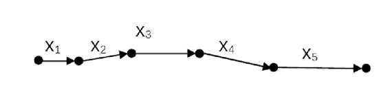
Fig. 1 . The graph for computational experiment

For such a graph, let us write down the continuity conditions (4)

^Z 1 ^{( l} 1 ) - ^Z 2 ⁽⁰⁾ = o , C 2 ⁽ l 2) - G⁽⁰ ) = ⁰ , ^Z 2 ^{( l} 3 ) - G⁽⁰ ) = ⁰ , ^Z 4 ^{( l} 4 ) ^{- Z} 5 ⁽⁰⁾ = ⁰

and the flow balance conditions (5)

Z ix (0) = 0 ,

^Z 1x ^{( l} 1 ) ^{— Z} 2x ⁽⁰⁾ = ⁰ ,

^Z 2x ^{( l} 2 ) ^{— Z} 3x ⁽⁰⁾ = ⁰ ,

^Z 3x ^{( l} 3 ) ^{— Z} 4x ⁽⁰⁾ = ⁰ ,

^Z 4x ⁽ l 4 ) ^{— Z} 5x ⁽⁰⁾ = ⁰ ,

^Z 5x ^{( l} 5 ) = ⁰ .

With the given coefficients β = 0 , 15, λ = 1 , 44, the Hoff equations will be set on the edges of the graph

• 1 ,    44 dζ j + dζ jxx = 0 , 15 ζ j dt + NdW j , j = 1 , 2 ,..., 5 .                 (12)

We will look for solutions ζ j ( t, x ) , j = 1 , 2 , ..., 5 of this problem in the form of Galerkin sums, by taking 7 summands.

ζ j ( t,x ) =       a k ( t ) ϕ j,k ( x ) , j = 1 , 2 , ..., 5 .

k=1

Having solved the Sturm–Liouville problem, we get

^A k = 25 ^, ^ 1,k (x) = }/ 15П + 1/ n c ^cos ( 15 x ) ^, ^ 2,k ( x ) = 1^ ^cos ( 15 (x ^{+ n )} ) , ^ 3,k ^{( x )} = I5 n c ^cos ( k (x ^{+ 3 n )} ) , V 4 ,k ^{( x )} = 1/ i c ^cos ( 15 (x ^{+ 6 n )} ) ^, ^ 5,k ^{( x )} = У^П ^cos ( k (x + ^{10 n )} ) .

Note that A = A ₆ . Thus, A ₆ G a L ( M ). According to the analytical investigation of the Hoff model of deformation in a structure of I-beams with an initial-final condition, let us assume that A 1 , A ₂ , A 3 , G ^ L (M ) and A 4 , A ₅ , A 7 G a L1 ( M ).

We will assume that the system is exposed to the same effect, therefore all random variables here are normally distributed Gaussian quantities ~ N (0; 0 , 6). Using the initialfinal conditions, let us obtain a representation for the initial values considered as follows

P o (Z (0) - ( o ) = E    (0 ,x ) - C o ( xU k Ы = 0 ,             (13)

k:µ _k ∈ σ ^L 10(M)

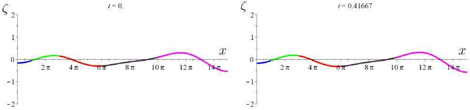
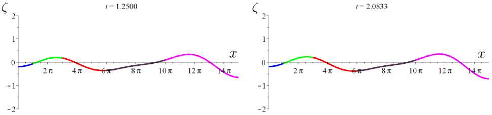
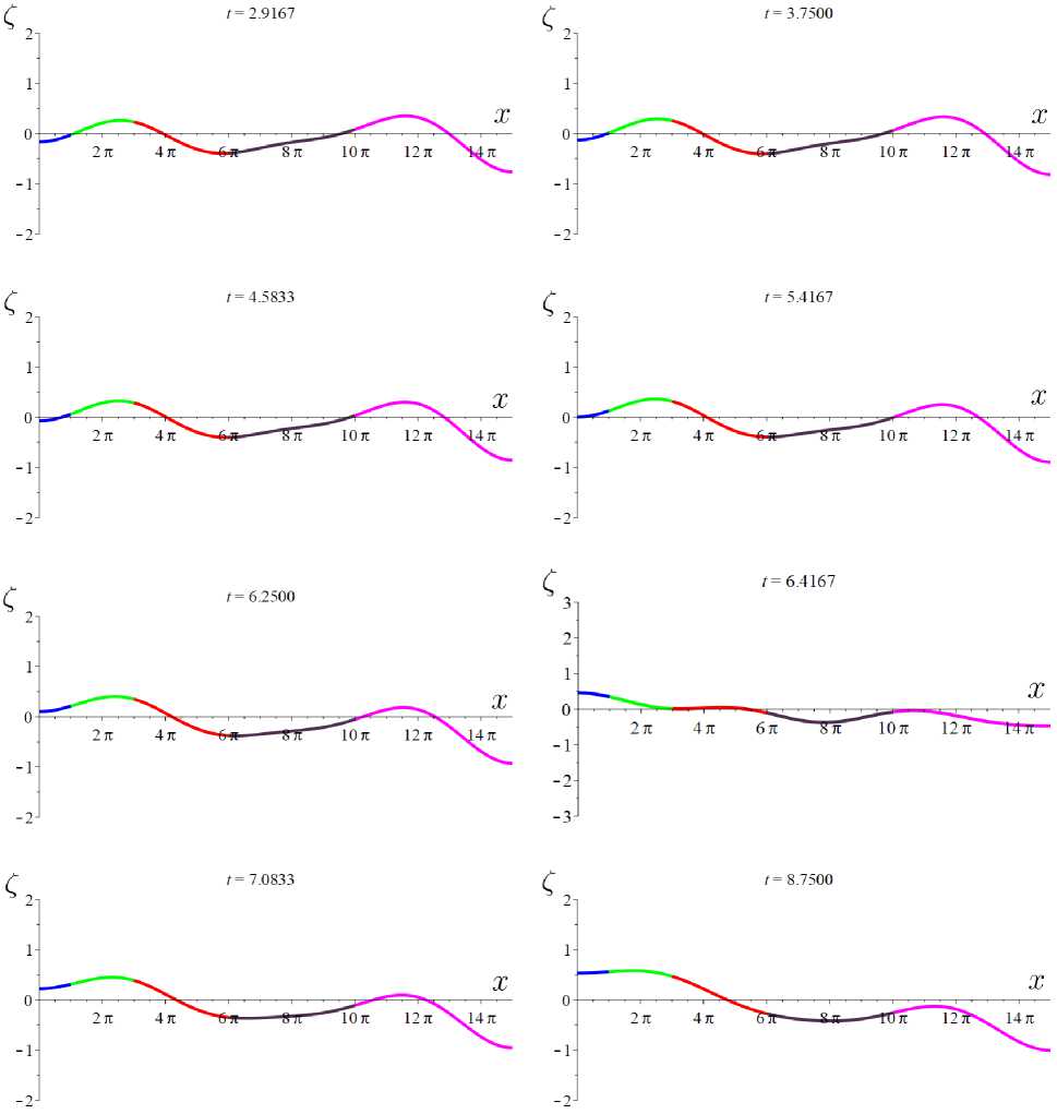
Pi(z(0) - б) = E   

k:λk∈σ₁^L₁(M)

further ξτ = (ξ1,0, ξ2,0, ξ3,0, ξ4,0, ξ5,0) and ξ1 = (ξ1,1, ξ2,1, ξ3,1, ξ4,1, ξ5,1) according to the number of edges j = 5.

As a result of the generation of random variables included in the decomposition for the functions of the initial condition, we obtained

(1,01 = -1, 57203253,   (1,o₂= -0, 6534010832, (1,o₃= -0, 01797861729,

ξ2,0₁= 0, 769351807,    ξ2,0₂= 0, 1959283956,    ξ2,0₃= 0, 1276538831,

ξ3,0₁= 0, 4600965754,   ξ3,0₂= 0, 05775170542,  ξ3,0₃= 0, 4919564389,

(₄,₀1 = -0, 2374773235, (₄,₀2 = 0, 00273696281,   (₄,₀3 = 0,491218275,

(₅,o1 = 0,470553412,    (5,02 = 0, 5003177325,    (5,03 = -0,4645654522.

By generating random variables that are part of the decomposition for the initial functions of the final condition, we obtained

(i,i4 = -0, 3283899452,  (1,15 = 0, 8185883182,     (1,17 = 0, 7807642225,

(₂,14 = 0, 206083644203,  (2,15 = -1, 36940970662, (217 = -0,187482338909,

(3,14 = 0,4579221402,    ^ = 0,4316586561,    (3,17 = -0, 2344698016,

(4,14 = -0, 05175526728, (4,15 = 0, 2550668598,     (4,17 = -0, 9918095115,

(5,14 = 0,11864946,       (5,15 = 1, 749752786;      (5,17 = -0, 2830376578.

The external effect on each edge may be represented by decomposition

NdWj = A sin(wt)φ1ϕ1 (x) + A sin(wt)φ2ϕ2(x) + A sin(wt)φ3ϕ3 (x)+ +A sin(wt)φ1ϕ4(x) + A sin(wt)ϕ5(x) + A sin(wt)ϕ7(x)

with A = 0, 765405620436, w = ¹₆, φk = (φ1_k, φ2_k, φ3_k, φ4_k, φ5_k) in accordance with the number of edges j = 5.

The generation of random variables included in the decomposition for random external action gave the following results:

φ11 = 0, 2246948044, φ12 = 1, 36697483468, φ13 = -0, 02737836647, φ14 = 0, 8498896526, φ15 = -0, 3518854196, φ17 = 0, 07826279773, φ21 = 0, 08735263553, φ22 = -0, 931286038, φ23 = -0, 1017266735, φ24 = -0, 2982196884, φ25 = -0, 5344867959, φ27 = -0, 03159215838, φ31 = -0, 2212717272, φ32 = 0, 7903122257, φ33 = 0, 6887758545, φ34 = 0, 03068167176, φ35 = -0, 7041800119, φ27 = -0, 6699585179, φ41 = 0, 4722770182, φ42 = -0, 2433091863, φ43 = 0, 04289751467, φ44 = -0, 5012154257, φ45 = 0, 297270174, φ47 = 0, 9044232645, φ51 = 0, 0272506223, φ52 = 0, 2489458583, φ53 = -0, 04979900558, φ54 = -0, 2764538139, φ55 = 0, 5463800986, φ57 = -0, 3528926737. The first system of differential equations with initial conditions contains three equations and three initial conditions. The second system of differential equations contains three equations and three final conditions for τ = 10. Obtained was one algebraic equation, the sixth one (since the sixth eigenvalue equals λ).

The first system da1 (t) - 0, 15a (t) - 0, 063296358 sin 0, 166667t = 0, dt             1

da (t)

0, 9955555556 _d²_t   - 0, 15a2(t)-

• -8, 17168916 · 10^-16cos(0, 166667t) - 0, 27851468 sin(0, 166667t) = 0,

  0, 982222222 ^da_d³_t^(t)- 0, 15a3(t)+

  • -2, 04292229 · 10^-15cos(0, 166667t) - 0, 044257363 sin(0, 166667t) = 0,

with conditions a1 (0) = -0, 376410562, a2 (0) = 0, 0164114362, a3(0) = 0, 0862050486.

The second system

• 0, 97^da4(t)- 0, 15a (t)-

• dt            4

• -1, 09101285 · 10^-15cos 0, 166667t + 0, 248536829 sin 0, 166667t = 0,

  0, 928888888 ^da5(t)- 0, 15a5(t)+

dt

+4, 11751779 · 10^-16cos 0, 166667t - 0, 30034281 sin 0, 166667t = 0,

0, 8888888 da7(t) - 0, 15a7(t)- dt

• -1, 10136402 · 10^-16cos 0, 166667t - 0, 197981101 sin 0, 166667t = 0,

with conditions a4(10) = -0, 748694532, a5(10) = 0, 263697458, a7(10) = -0, 069132153.

Algebraic equation has the form a6 (t) = 0, a6(0) = 0.

Next, we combine and solve the two systems, after which an approximate solution to the initial-final problem is found on the graph in question. The analytical result is rather cumbersome; therefore, the results of the computational experiment are presented graphically (Figs. 2 – 4) in the form of two-dimensional graphs at various points in time t^∗. The abscissa axis reflects the values of the variable x and reflects the length of the edges of the graph. The ordinate axis reflects the values of the Zj (x,t*) function: the dynamics of buckling of I-beams in a structure under constant load with random external effect.

The colors show solutions on different edges of the graph: Z1(x,t*) — blue, Z2(x,t*) — green, Z₃(x,t*) — black, Z4(x,t*) — red, Z5(x,t*) — magenta.

The sequence of graphs reflects the development of the process over time, taking into account the structure of the graph. Of note, the curve of the graph characterizes the deviation of the I-beam from the vertical on the corresponding edge of the graph.

Fig. 2. Results of computational experiment

Fig. 3. Results of computational experiment

Fig. 4. Results of computational experiment