Optimal Control Approach for Solving Linear Volterra Integral Equations

Published Online April 2012 in MECS

Volterra integral equations arise in many physical applications, e.g., potential theory and Dirichlet problems and electrostatics. Also, Volterra integral equations are applied in the biology, chemistry, engineering, mathematical problems of radiation equilibrium, the particle transport problems of astrophysics and reactor theory, and radiation heat transfer problems [1,2,3,4,5]. There exist the some valid approximate and numerical methods for solving Volterra integral equation such as Adomian decomposition method [6], Walsh functions method and multigrid approach [7, 8], Bernstein Polynomials method [9], collocation method [10,11,12,13,14,15], Langrange interpolation method [16], Taylor-series expansion method [17,18,19], classical Neumann-series method [20], spectral methods [21,22,23,24,25,26,27], finite element method [28], Sinc method [29,30], Galerkin method [31,32], wavelet approach [33], block-by-block method [34] and homotopy analytic method [35,36,37,38,39].

In this paper, we present a different approach from above methods for solving linear volterra integral equations which is based on the optimal control theory [40,41,42]. Consider the following linear Volterra integral equations of second kind:

x

a where a and b are constant, functions g(.,.) and ф(.) are continuously differentiable with respect to x . In equation (1), functions ф(.) and g(.,.) are known and y (.) is an unknown function. We assume that equation (1) have a solution.

The structure of this paper is as follows: Section 2 shows that solving Volterra integral equation (1) is equivalent to solve several optimal control problems. In section 3, a discretization method is applied to convert the problem to the corresponding linear programming problem. In section 4, the applicability of the approach is illustrated in several examples in which the computed results are compared with the exact solution. Section 5, gives the conclusion of this paper.

• II.    Optimal control problems

In this section, we are going to introduce some optimal control problems corresponding Volterra

dg equation (1). Let p =—. By using Leibnitz 9x derivatives we have:

d-Tg (x, t) y (t) dt = g (x, x) y (x) dx a integral

rule for

+ [ p ( x , t ) y ( t ) dt .

a

Also from equation (2) and differentiating both sides of (1) respect to x we have:

x                                         (3)

a

Now let x e [ a , b ] be an arbitrary given number. We define the following problem:

y ' ( z ) = ф'(z ) + g ( z , z ) y ( z ) + v ( z ),    z e [ a , x ] (4)

’ £ ( v ' ( t ) - p ( z , t ) y ( t ) ) dt = 0, z e [ a , x ]            (5)

_ y ( a ) = ф ( a ), v ( a ) = 0.                                  (6)

Theorem II.1: Let x e [ a , b ] be an arbitrary number and

( y * (.), v * (.) ) be solution of problem (4)-(6). Then we have:

x

a

Proof: Let x e[a, b ] . By initial conditions (6) and equation (5), we obtain

So, by using equation (8) and (4), we take y *'( z) = фХz) + g (z, z) y * (z)

+     p ( z , t ) y * (t ) dt ,       z e [ a , x ]

a

Hence

У *( z ) = Ф ( z ) + d-V g ( z , t ) y * (t ) dt , z e [a , x ]. dz ^a

By integrating both sides of above equation on [a,x]

and conditions (6), we obtain the equation (?).□

Now, let x e[a,b ] be an arbitrary given number and define the following optimal control problem:

Minimize fx |ф'(t) + g(t,t)y (t) + v (t) -u 1(t )|dt fx Ф'(z) + g (z,z)y * (z) + v * (z) - y' (z )|dt = 0.

Hence

*

y ^(t ) = Ф ^(t ) ⁺ g^(t , t ) y ^(t ) ^{+ v (t} ) .

Moreover, equation (5) and initial conditions (6) hold for pair (y * (.),v * (.)) . Thus, pair (y * (.),v * (.)) is the solution of the problem (4)-(6) and this completes proof. □

Now let n eN be a given large number. Set x ₀ = a ,

b - a h = and x. = a + jh for j = 1,2,...,n. The nj corresponding optimal control problem (9) for x = x

j

subject to

j = 1,2,..., n is as follows:

y'(t ) = u /t ), t e [ a , x ]                   (9)

v ' ( t ) = u ₂( t ), t e [ a , x ]

r(t , y , u 2 ) = 0, t e [ a , x ]

y ( a ) = ф ( a ), v ( a ) = 0, where ( y (.), v (.) ) and ( u 1 (.), u 2 (.) ) are state and control variables, respectively, and for t e [ a , x ]

r(t , y , u 2 ) = £( u 2 (w ) - p ( t , w ) y ( w ) ) dw . (10) Theorem II.2: Let x e [ a , b ] be an arbitrary given number and pairs ( y * (.), v * (.) ) and ( u 1 * (.), u ₂ * (.) ) be optimal state and control of the problem (9), respectively. Then function y * (.) satisfies equation (7).

Proof: Assume that x e [ a , b ] is an arbitrary given number. By theorem II.1, it is sufficient that we show pair ( y * (.), v * (.) ) is the solution of problem (4)-(6). Define the following problem corresponding to the problem (9): Minimize

J(y,v) = £ Ф(t)+ g(t,t) y(t)+ v (t) -y't )dt(11)

subject to

{(v'(w) - p (t,w)y (w))dw = 0, t e [a, x ](12)

y (a) = ф(a), v (a) = 0.(13)

Now, let y (.) = y (.) be the solution of the equation (1), and v (.) = v (.) satisfies equation (12) where y (.) = y (.) . It is trivial that pair ( y * (.), v * (.) ) satisfies initial conditions (13) and J ( y , v ) = 0 . On other hand, since ( y * (.), v * (.) ) and ( u 1 * (.), u ₂ * (.) ) are optimal solutions of problem (9), pair ( y * (.), v * (.) ) is the optimal solution of the problem (11)-(13) and we have J ( y * , v * ) = 0 . Thus

Minimize

{xj |ф'(t) + g(t,t)y (t) + v (t) -u 1(t )|dt subject to y'(t) = ui(t), t e[a,xj ]                (14)

v ' ( t ) = u ₂( t ), t e [ a , x j ]

r(t,y,u2) = 0, t e[a,xj ] y (a) = ф(a), v (a) = 0, where r (.,.,.) is defined by (10). We rewrite problem (14) for j = 1,2,...,n as follows:

Minimize

Efx‘ |ф'(t)+g(t,t)y(t)+ v (t)-u 1(t)ldt k=1 k -1

subject to y '(t) = u 1(t), t e[xk-1,xk ], k = 1,2,...,j (15) v'(t) = u2(t), t e[xk-1,xk ], k = 1,2,..., j r(t,y ,u2) = 0, t e[xk-1,xk ], k = 1,2,..., j y(x0) = Ф(x0), v(x0) = 0.

By assumption

^ ( t ) = Ф ( t ) + g (t , t ) y (t ) + v ( t ) - u 1 ( t ) , t e [ a , b ] the problems (15) for all j = 1,2,..., n is equivalent to the following multi-objective programming problem:

Minimize(

{j1 Ф( z) dz, j1 фсz) dz + j 2 фсz) dz, 0                            01

..., fx1 Ф( z) dz +{x2 ф( z) dz +...+fx n ф( z) dz} Jx0                      x 1

subject to     y'(t) = u,(t), t e [xk_,,xk ], v '(t ) = u 2(t ), t e [ xk-1, xk ], r(t,y,u2) = 0, t e [xk-1,xk ], y (x 0) = Ф( x 0), v (x 0) = 0, k = 1,2,..., j , j = 1,2,..., n.

By multi-objective programming methods (see [43]), we can use the following problem instead of problem (16): Minimize

J = ^ (n - к +1)f k |w(z )|dz(17)

к =1■ subject to

У'(t) = u 1(t), t €[Xk-1,Xk ], к = 1,2,...,n (18) v '(t) = u 2(t), t €[ xk -1, xk ], к = 1,2,..., n,

r(t,У,u2) = 0, t e[xk-1,Xk ], к = 1,2,...,n (20) У (x0) = ф(x0), v (x0) = 0.

Define the following problem for к = 1,2,..., n :

Minimize

Jk = (n - к + 1)f k Wz )|dz(22)

J ^x k - 1

subject to

У '(t) = u,(t), t e[Xk-1,Xk ], v '(t) = u2 (t), t e[Xk-1,Xk ], rk -1(t, У,u 2) = 0, t e[Xk-1, Xk ],

y(Xk-1) = y[k-1],v(Xk) =v[k-1].

where y ^{[ k - 1]} and v ^{[ k - 1]} are known numbers which we can obtain these numbers by solving problem (22)-(26) on interval [ x _{k - 2}, x _{k - 1}] . Moreover, for t e [ x _{k - 1}, x _k ]

r k - 1 ^{( t} , У , u 2 ) = f t ( u 2 ⁽ w ) - P ⁽ t , w ) У ⁽ w ) ) ^dw .

* ^Xk - 1

Now we have the following theorem:

Theorem П.3: Let     ( y * _k _ ,) (.), v *_k _ ,) (.) ) and

( u ( _{k - 1} ) ₁(.), u ( k _{- 1} ) ₂(.) ) for any k = 1,2,..., n be optimal state and control of problem (22)-(26), respectively. Then optimal solutions of problem (17)-(21) are as follows:

y,(t) = у(к-1)(t), te[xk-1,xk], k = 1,2,...,n v *(t) = v(k-1)(t), t e[Xk-1,Xk ], к = 1,2,...,n u1*(t) = u(к-1),1(t), t e[xk-1,xk], k = 1,2,...,n u2(t ) = u (к -1),2(t X t e[Xk -1, Xk ], k = 1,2,..., n.

Proof: Consider the following sets:

D = {( У , v , u ₁, u ₂): ( У , v , u ₁, u ₂) satisfies in equations

(18)-(20) on [ x 0 , x n ] },

D_k = {( y , v , u ₁, u ₂):( y , v , u ₁, u ₂) satisfies in equations (23)-(26) on [ X k - 1 , X k ]} , k = 1,2,..., n

n

It is trivial that D = ^D, . In addition, the value of k =1 k objective functional in problems (17)-(21) and (22)-(26)

are nonnegative. Thus, we have:

n

Minimize J = V (Minimize Jk )

( y , ^v , и 1 , и 2^{) e} D           k"= 1 < У - ^v - ^u 1 , ^u 2^{) e D} k

The system (27) is immediate from latter relation and optimality principle in continuous-time dynamic programming which initiated by Bellman (see section 8 of [44]). □

Remark II-4: Note that y ^[0] = ф ( x ₀) and v ^[0] = 0 .

• III.    Linear programming problems

In this section, we convert the continuous problem (22)(28) to an equivalent discrete problem and solve the obtained problem by linear programming method (see [45]). For this purpose, consider the following approximations in numerical differentiation and integration for k = 1,2,..., n and t = x_{k - 1}, x_k :

f ^r‘ | a ( z )| dz « h (| w ( ^x k _ ₁⁾| + | a ( ^x k ) )

* ^Xk - 1                     2

У '(t) “1 (У (xk) - У (xk -1)),    v '(t) «1 (v (xk) -v (xk _,)), hh f k (u2(w )- p(xk,w )y (w ))dw »

x k - 1

h 2 ( ^u 2, k - 1 - P ( ^X k , ^X k - 1 ) У к - 1 ^{+ u} 2k - P ( ^X k , ^X k ) У к ) .

Using the above approximation we can transform problem (22)-(28) to the following corresponding problem for k = 1,2,..., n :

Minimize

Jk = h2(n - k +1)(|Wk-J + |Wk I)

subject to

^y k - ^y k - 1 - ^hu 1,k - 1 = 0, ^y k - ^y k - 1 - ^hu 1,k = 0, ^v k - ^v k - 1 - ^hu 2, k - 1 = 0, ^v k - ^v k - 1 - ^hu 2, k = 0, ^u 2, k - 1 - P ^{( x} k , ^x k - 1 ) У к - 1 ^{+ u} 2, k - P ^{( x} k , ^x k ) У к = ⁰,

^[ k ^{- 1]}, v- , = v ^{[ k - 1]}

where for l = k - 1, k we have:

u 1, l    u 1 ^{( X}l ), u 2, l    u 2 ^{( X}l ),

W i = W ^{( x} l ), У I = У ^{( x} l ), ^v l = ^{v ( x} l ).

Now by applying the techniques of linear and nonlinear programming [45,46], and relation

W ( t ) = ф (t ) + g ( t , t ) y ( t ) + v (t ) - u 1 ( t ), t e [ a , b ] the nonlinear problem (28) be converted to the following corresponding linear programming problem for k = 1,2,..., n :

h

Minimize Jk = —(n - k +1)(zk-1 + zk) (29)

subject to

W k - 1 ⁺ z k - 1 ^ ⁰, - W k - 1 ⁺ z k - 1 ^ ⁰,

Wk + zk ^ 0, - Wk + zk ^ 0,

g ^{( x} k - 1 , ^x k - 1 ) У к - 1 ^{+ v} k - 1 - ^u 1,k - 1 - W k - 1 =- ф ^{,( x} k - 1 ),

g ^{( x} k , ^x k ) У к ^{+ v} k - ^u 1,k - W k =- ф ^{,( x} k ),

У к - У к-1 - hu 1, к-1 = 0, У к - У к-1 - hu 1,к = 0, vk - vk-1 - hu 2k -1 = 0, vk - vk-1 - hu 2, k = 0, u 2,k -1 - P (xk ,xk -1) Ук -1 + u 2,k - P (xk ,xk ) Ук = 0,

Ук-1 = У [k-1], vk-1 = v[k-1],zk-1 ^ 0,zk ^ 0, where decision variables of this problem are zz, ц1, y t,v z, u 1z and u 2l for l = k -1, k . Not that by solving problems (29), we obtain the approximations y* , k = 1,2,...,n for exact solution of problem (1), meansy *(x k), k = 1,2,...,n .

Remark III.1: Note that, in this approach, we solve the linear programming problem (29) and use theorem 2-3 to approximate the solution of equation (1).

In next section, we illustrative the efficiency of our approach in some numerical examples.

• IV.    Simulation results

In this section, we use our approach to solve two linear Volterra integral equations. Here we apply the MATLAB software and simplex method [45] for solving linear programming problem (29).

Example IV.1 : Consider the following Volterra integral equation of second kind:

^x 2 + cos( x )

y ^{( x} ) = e sin ^x ) +1 ------ -^y (t ) d , ^J° 2 + cos( t )              (30)

_ x G [0,1].

The exact solution of equation (34) is y (x) = ex sin(x)

+ e^x (2 + cos( x ))(ln(3) - ln(2 + cos( x ))), Here for n = 10,20,50 and n = 100 , we solve corresponding problem (29) for equation (30). In Figures 1-4, the connected line indicates the graph of exact solutions. The comparison of obtained results and exact solution for equation (29) are showed in Table 1.

Example IV.2: Consider the following Volterra integral equation of second kind:

y ( x ) = sin( x ) +[ 2cos( x - 1 ) y (t ) dt ,

)                            J0

_ x g [0,1].

Here for n = 10,20,30 and n = 40 , the corresponding problem (29) for equation (31) is solved. The connected line indicates the graph of exact solutions. We can compare the obtained results and exact solution of equation (31) in Table 2.

• V.    Conclusions

In this paper, we obtained optimal control problems corresponding Volterra integral equation. By discretization method these optimal control problems converted to the corresponding linear programming problems. Thus we can solve linear programming problems instead of Volterra integral equations. By this approach, we can obtain a good approximation for the solution of linear Volterra integral equation.

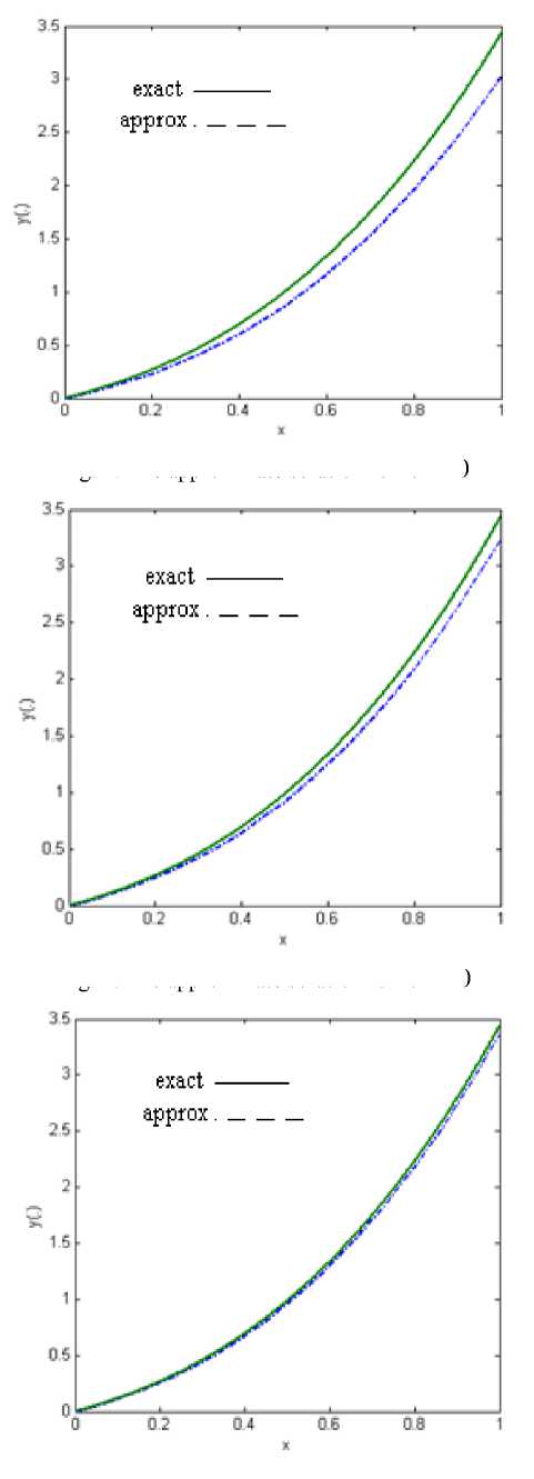
Fig .3: The approximate solution for n = 50

Fig. 1: The approximate solution for n = 10

Fig. 2: The approximate solution for n = 20

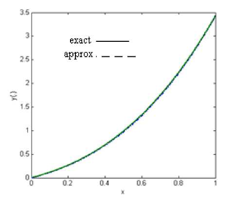
Fig. 4: The approximate solution for n = 100

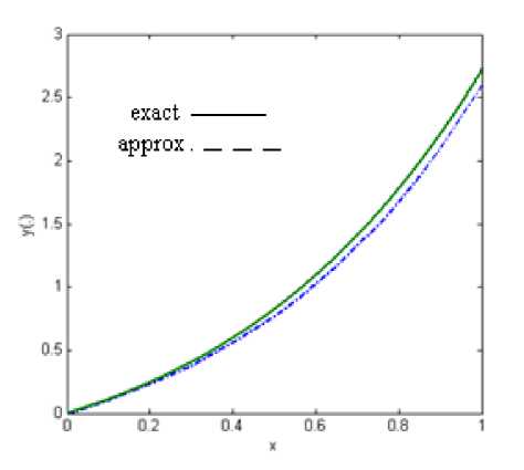
Fig. 6: The approximate solution for n = 20 .

Table 1: Comparison of exact and approximate solutions for Ex. IV.1 .

x	Approximate solution for n =10	Approximate solution for n =20	Approximate solution for n =50	Approximate solution for n =100	Exact solution
x =0.2	0.23098159	0.24826681	0.25929638	0.26309086	0.26692094
x =0.5	0.86113061	0.92262360	0.96197727	0.97553724	0.98809616
x =0.8	1.96419901	2.09898018	2.18542479	2.21524535	2.21524535

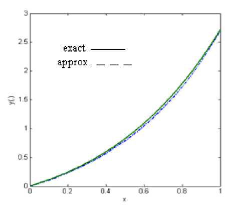
Fig. 7: The approximate solution for n = 30

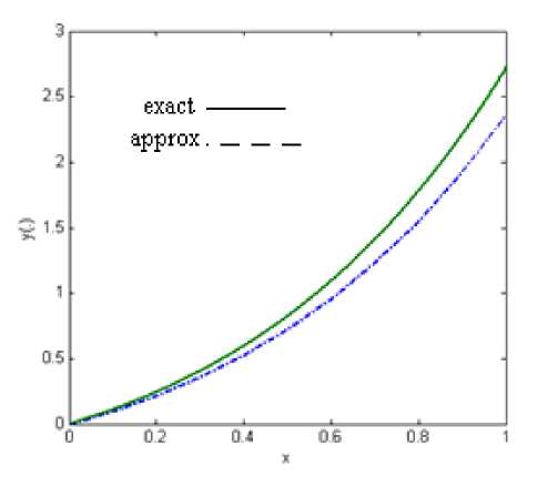
Fig. 5: The approximate solution for n = 10 .

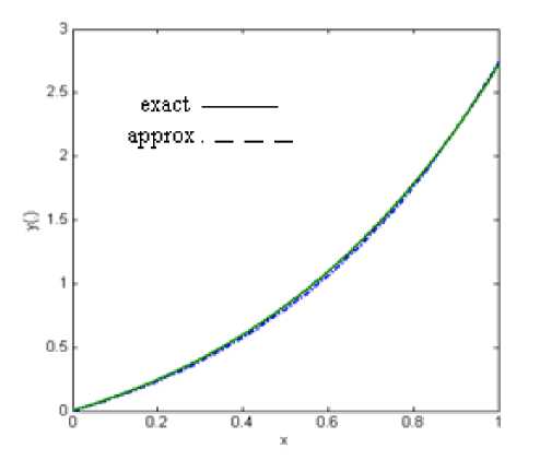
Fig. 8: The approximate solution for n = 40

Table 2: Comparison of exact and approximate solutions for Ex. IV.2 .

x	Approximate solution for n =10	Approximate solution for n =20	Approximate solution for n =30	Approximate solution for n =40	Exact solution
x =0.2	0.21950041	0.23111194	0.23534042	0.23753096	0.24428055
x =0.5	0.72596658	0.77435737	0.79243764	0.80190046	0.82436063
x =0.8	1.54942048	1.68180727	1.73246743	1.75923588	1.78043274