Parameter Tuning via Genetic Algorithm of Fuzzy Controller for Fire Tube Boiler

Published Online April 2012 in MECS DOI: 10.5815/ijisa.2012.04.02

The fire tube boiler has been used extensively for the generation of energy in a wide range of industrial processes and heating applications. The requirements of an efficient boiler are that should generate maximum amount of steam at a required pressure, temperature and quality with minimum fuel consumption. To achieve optimal design, a precise control system design is required. Sufficient and trustworthy information about dynamics properties of the plant is the basis for successful control system design.

Boiler control is the regulating of the boiler outlet conditions of steam demand, pressure, and temperature to their desired values. At the same time, regulating boiler internal parameters such as water level is very important to keep the boiler safely. The quantities of fuel, air, and water are adjusted to obtain the desired steam demand and maintain the steam temperature and water level inside shell at their set point. The studies of dynamics of fire tube boilers and control systems have been studied rarely in the past. Only few simple lumped SISO models for domestic fire tube hot water heater appeared in literature [1], [2], [3], [4], and [5].

Unlike water tube boiler which has been studied extensively in the past [6], [7], [8], [9], [10], and [11].The closed loop control problem of the process is investigated, where high static accuracy and high speed of response with no overshoot are required as a technical design criterion.

Different control polices such as Fuzzy control and Genetic-Fuzzy control can be applied and tested for applicability under certain operating conditions, or subjected to some constraints.

The theory of fuzzy sets [12] becomes a useful instrument for control engineer as the complexity of the system increases and the ability to understanding and predicts its behavior in a precise and yet significant manner diminishes.

Genetic algorithms are global, parallel, search and optimization methods; founded on Darwinian principles [13] and [14], which based on analogies to natural biological processes.

However, designing a robust control system, which provides performance specifications and guarantee closed loop stability irrespective to parameters variations is appraising target attracting many control designers and researchers.

The effect and violability of the Genetic-Fuzzy control system and comparison with conventional control methods such as Fuzzy control are investigated by nonlinear dynamic model simulation.

The paper has been organized as follows: Section 2 describes the system dynamic model. Section 3 reviews the FLC tuning method. Section 4 presents the design method of GA while section 5 explains how GA can tune FLC. Section 6 illustrates the simulation results of the proposed controller. Finally, a conclusion of the proposed GFLC technique is presented in Section 7.

II. MATHEMATICAL MODEL

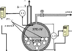
There are two feedback control loops, water/steam temperature control loop, and water level control loop. The schematic diagram for the fire tube boiler control system is shown in Fig. 1. In our case, the process is 2-input 2-outpu multivariable process with interaction between the two feedback closed loops. The input fuel flow rate m f , will act as control for water/steam temperature T_w , but will act as a disturbance for water level hw, where m w represents the feed water flow rate. Both control loop operate on its own and interacts with the other loops.

	C 16 + C 11 C 4	C 7 + C 12 C 4	0	0
	M C g	Ms C g
	C 6	h mw A mw — C /	h mw A mw	0
	M m C m	M m C m	M m C m
A =	0	C 14 h mw A mw	C 14 ( h mw A mw + UA + C>)	0
		C 14 C 17 - C 16 C 15	C 14 C 17 - C 15 C 16
	0	C 16 h mw A mw	C 16 ( h mw A mw + UA + C 9 )	0
		C 14 C 17 - C 15 C 16	C 14 C 17 - C 15 C 16

C 1 - C 13 - C 4 C 13            0

M g C g

0 C 14 C 19 - C 5

C 14 C 17 - C 16 C 15

0               C 5 - C 16 C 19

C 14 C 17 - C 16 C 15

C 2 - C 5

M g C g

Flue gases

Set point, Tw

Fire Tubes

Set point, hw

Fuel flow rate

Steam outlet

and

Feed water inlet

Fig. 1. A schematic diagram for fire tube boiler control system

The first step in the analysis of a dynamic system is to drive its mathematical model of the plant. The dynamic model of a fire tube boiler [15] is considered, as previously derived, using heat transfer, mass balance, and heat balance equations, and can be modeled as:

X = Ax + Bu + Efd . y = ex ;

The state vector x, the manipulated input vector u, the output vector y, and the disturbance input vector fd are defined as:

x = T

~~~

T m T w V w ]

u

~ m w ]

f d = [ m⁵

T o ] ^T ;

y

= [ t w

~ T h w ]

C 14 C 18 + C 15           C 14 UA

C 17 C 14 - C 16 C 15 C 17 C 14 - C 16 C 15

C 16 C 18 + C 17           C 16 UA

C 17 C 14 - C 16 C 15 C 17 C 14 - C 16 C 15

C =

III. FUZZY LOGIC CONTROLLER

The main idea of the fuzzy logic controller (FLC) is the measured value is a crisp quantity fuzzified into a fuzzy set. This fuzzy output is then conceded as the fuzzy input into a fuzzy controller, which is consisted of linguistic rules. The output of the fuzzy controller is then another series of fuzzy sets. Since most physical system cannot interbreed fuzzy commands (Fuzzy Sets), the fuzzy controller output must be converted into crisp quantities using defuzzification methods.

The crisp (defuzzified) control output values then become the input values to the physical system and entire closed loop cycle is repeated. As shown in Fig. 2, the control inputs u derive the process variables y for both control loops.

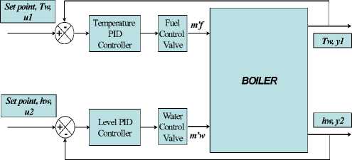
Figure 2 ． The block diagram for fire tube boiler control system

• A.    Water/steam temperature control loop

For temperature fuzzy logic controller, we use a Mamdani fuzzy controller. The temperature error is fuzzified and will be used as the input to fuzzy controller. The membership functions for both input and output fuzzy variables are triangle shaped functions and symmetrical about zero [16], as shown in fig. 3.

The temperature error, “e”, will be fuzzified by five linguistic variables, “NL” stands for “negative large”, “NS” for “negative small”, “Z” for “zero”, “PS” for “positive small” and “PL” for “positive large”, partitioned on the error space. For the controller output, control quantity “z”, will be described by five linguistic variable labeled CLOSEFAST, CLOSESLOW, NOCHANGE, OPENSLOW, and OPENFAST partitioned on control universe.

A number of rules are used to model the way of the system behavior; fuzzy rules are constructed in the well-known IF-THEN form. Five fuzzy rules base used for the temperature fuzzy controller are

IF (“e” is NL) THEN (“z” is CLOSEFAST). IF (“e” is NS) THEN (“z” is CLOSESLOW). IF (“e” is Z) THEN (“z” is NOCHANGE). IF (“e” is PS) THEN (“z” is OPENSLOW). IF (“e” is PL) THEN (“z” is OPENFAST).

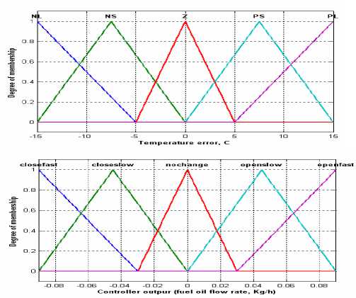
Figure 3. Temperature fuzzy logic controller membership function

The fuzzy logic control rules were formulated trial and error by making correction to the rule base after examining the system response. The desired response was the quickest rise time with no overshot and smooth damped rise. The large membership functions have a relatively small domain and are presented to deliver relatively large control inputs when the error is at extremes, this essential for the quick response time to the step input. The small membership functions have a relatively large domain and are presented to deliver relatively small control inputs when the error is around zero, this for no overshot response.

A defuzzification method is required to transform fuzzy control output to a crisp value of the fuzzy logic controller. For the temperature FLC, a widely used defuzzification method is the “center of area”.

At each time step, the FLC examines the change in water/steam temperature from the set point, temperature error, these data are crisp quantity, and must be fuzzified and given as input to inference engine. Utilizing the current set of rules, a fuzzy control output representing the change in fuel flow rate is defuzzified and applied to the plant.

• B.    Water level control loop

For level fuzzy logic controller, we use a Mamdani fuzzy controller. The level error fuzzified and will be used as the input to fuzzy controller. The membership functions for both input and output fuzzy variables are triangle shaped functions and symmetrical about zero [16], as shown in Fig. 4.

The level error, “e”, will be fuzzified by five linguistic variables, “NL” stands for “negative large”, “NS” for “negative small”, “Z” for “zero”, “PS” for “positive small” and “PL” for “positive large”, partitioned on the error space. For the controller output, control quantity “z”, will be described by five linguistic variable labeled CLOSEFAST, CLOSESLOW, NOCHANGE, OPENSLOW, AND OPENFAST partitioned on control universe.

A number of rules are used to model the way of the system behavior; fuzzy rules are constructed in the well-known IF-THEN form. Five fuzzy rules base used for the level fuzzy controller are

IF (“e” is NL) THEN (“z” is CLOSEFAST). IF (“e” is NS) THEN (“z” is CLOSESLOW). IF (“e” is Z) THEN (“z” is NOCHANGE). IF (“e” is PS) THEN (“z” is OPENSLOW). IF (“e” is PL) THEN (“z” is OPENFAST).

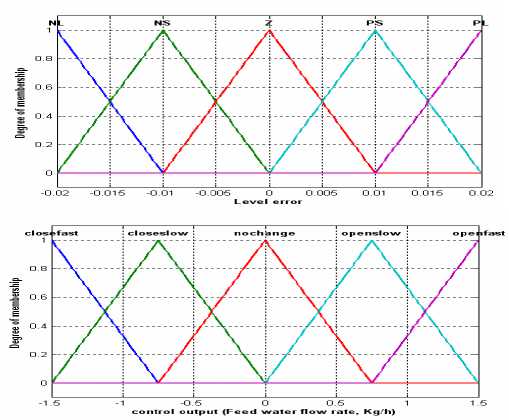
Figure 4. Water level fuzzy logic controller membership function

The fuzzy logic control rules were formulated trial and error by making correction to the rule base after examining the system response. The desired response was the quickest rise time with no overshot and smooth damped rise. The large membership functions have a relatively small domain and are presented to deliver relatively large control inputs when the error is at extremes, this essential for the quick response time to the step input. The small membership functions have a relatively large domain and are presented to deliver relatively small control inputs when the error is around zero, this for no overshot response.

A defuzzification method is required to transform fuzzy control output to a crisp value of the fuzzy logic controller. For the level FLC, a widely used defuzzification method is the “center-of-area”.

At each time step, the FLC examines the change in water/steam level from the set point, temperature error, these data are crisp quantity, and must be fuzzified and given as input to inference engine. Utilizing the current set of rules, a fuzzy control output representing the change in fuel flow rate is defuzzified and applied to the plant.

In the fuzzy system, computational effort is spent in finding parameters that give a desired behavior to the system, while no attention is given to the structure of the system because the control engineer is looking for a good enough solution not necessary the optimum one. However, sometimes the parametric adjustment of the selected structure may be too poor.

Besides the large tuning time and the significant amount of wasted resources, the structure is too complex and the dimension of the problem increase unreasonably. Therefore, we will use optimization technique using Genetic algorithm to find the FLC parameter in order to save time and effort that spent in tuning the FLC parameter.

• IV. THE GENETIC ALGORITHM

In any design problem there is a multi-dimensional space of possible solutions. Some of these solutions may be acceptable, but not the best (local optimum) and there may exist a single best solution (global optimum). An alternative approach is to use “heuristics” or knowledge required through experience, to search for optimal solutions. One such technique is to employ a Genetic Algorithm (GA) [13] and [14].

The GAs is global, parallel, search and optimization methods; founded on Darwinian principles; the evolution is based on two simple concepts of natural evolution: “survival of the fittest” and “reproduction the basic element of a GA is the “chromosome”. It contains the genetic information for a given solution and is typically coded as binary string. GA operates on a set (population) of strings (individuals that represents a particular solution of the problem), where each string has input data. Each string’s fitness (which expresses how good the solution is at solving the problem) is calculating using an objective function.

In GA terminology, each iteration of the search is called a “generation”. In each generation, taking advantage of the fittest individuals of the pervious generation creates a new population.

GA is characterized by attributes such as objective function, encoding the input data, genetic operators, population size, and then the algorithm programming steps.

• A.    The objective and fitness function

The objective function is used to provide a measure of how individuals have performed in the problem domain. In the problem of a minimization problem (our case), the fit individuals will have the lowest numerical value of the associated problem objective function. This raw measure of fitness is usually only used an intermediate stage in determining the relative performance of individuals in a GA. Another Function, the fitness function, is normally used to transform the objective function value into a measure of relative fitness. A “fitness function”, which is in effect a performance index, is used to select the best solution in the population to be parents to the off springs that will comprise the next generation. This emulates the evolutionary process of “survival of the fittest”.

F(x)=g(f(x))               (2)

Where “f” is the objective function, “g” transforms the value of the objective function (f(x)) to a non-negative number and “F” is the resulting relative fitness, in the current study (3) is the chosen fitness function. This mapping is always necessary when the objective function is to be minimized.

• B.    Encoding

In a GA, each solution must be encoded as a binary sequence, i.e., a sequence of 0's and 1's. GAs operates on an encoding of the problem’s input data. The choice of the encoding is extremely important for the execution performance of the algorithm. A poor encoding can lead to long running searches that do not produce good results.

• C.    GA operator

GAs features the following three basic operators, which are executed sequentially by the GA:

• (1)    Selection and reproduction.

• (2)    Crossover.

• (3)    Mutation.

During the process of Selection and reproduction, pairs of individuals are chosen from the population according to their fitness. The reproduction operator can be implemented in a number of ways. For our purpose, in this paper roulette wheel was considered. The “roulette wheel” mechanism is probabilistically select individuals based on some measure of their performance. A real- valued interval, Sum, is determined as either the sum of the individuals’ expected selection probabilities or the sum of the raw fitness values over all the individuals in the current population. Individuals are then mapped one-to-one into contiguous intervals in the range [0, Sum]. The size of each individual interval corresponds to the fitness value of the associated individual.

For example, in Fig. 5, the circumference of the roulette wheel is the sum of all six individual’s fitness values. Individual 5 is the fit individual and occupies the largest interval, whereas individuals 6 and 4 are the least fit and have correspondingly smaller intervals within the roulette wheel. To select an individual, a random number is generated in the interval [0, Sum] and the individual whose segment spans the random number is selected. This process is repeated until the desired number of individuals has been selected.

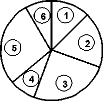
Figure 5. Roulette Wheel Selection

The basic roulette wheel selection method is stochastic sampling with replacement (SSR). Here, the segment size and selection probability remain the same throughout the selection phase and individuals are selected according to the procedure outlined above. SSR gives zero bias but a potentially unlimited spread. Any individual with a segment size > 0 could entirely fill the next population.

Crossover operators is used to combine the pairs of selected strings (parents) to create new strings (offspring) that potentially have a higher fitness than either of their parents. The crossover likes its counterpart in natural. Crossover operator can be implemented in a number of ways. For our purpose, the simplest recombination operator is that of single-point crossover. Consider the two parent binary strings as Fig. 6, If an integer position, I, is selected uniformly at random between 1 and the string length, L, minus one [1, L-1], and the GA information exchanged between the individuals about this point, then two new offspring strings are produced. The two offspring below are produced when the crossover point I = 5 is selected, this crossover operation is not necessarily performed on all strings in the population. Instead, it is applied with a probability P x , when the pairs are chosen for breeding.

01010011    01010110

11001110    11001011

Parents

Offspring

• Figure 6.    Single Point Crossover

  01010110    01110110

• Figure 7.    Binary Mutation Operator

A further GA operator, called Mutation, is then applied to the new chromosomes, every string resulting from the crossover process; gain with a set probability, P m . Mutation causes the individual genetic representation to be changed according to some probabilistic rule. In the binary string representation, mutation will cause a single bit to change its state, 0 ^ 1 or 1 ^ 0, and modified elements in chromosomes. Therefore, for example, Fig. 7, mutating the third bit leads to the new string, Mutation is generally considered a background operator that ensures that the probability of searching a particular subspace of the problem space is never zero. Therefore, the mutation operator is crucial and providing a guarantee to avoid missing high fitness strings when the current population has converged to a local optimum.

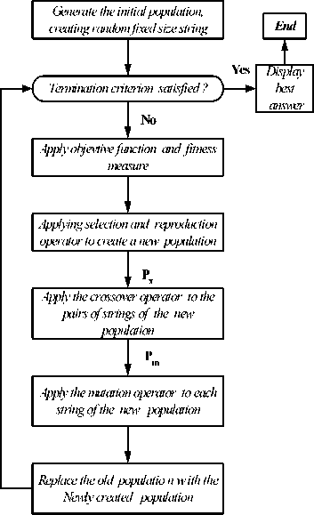
Fig. 8. Genetic programming flowchart

• d.    Population size

The number of string in a population is defined by the population size. The larger the population size, the better the chance that an optimal solution will be found.

• e.    How the algorithm works?

GAs uses the operator defined above to operate on the population through an iterative process as shown in fig.8, the GA is terminated when some criteria are satisfied, e.g. a certain number of generations, a mean deviation in the population, or when a particular point in the search space is encountered, in this paper we terminate the GA when the certain number of generations are satisfied.

• V. GFLC CONTROLLER DESIGN

The GA used as an optimization technique to find the optimal FLC parameter, in Fig. 9, shows the technique of the GA works in tuning the FLC parameter. The objective function block used for calculating the FLC performance. The Genetic algorithm block used for finding the optimized FLC parameters to locating the optimal solutions of the controller output “u” to meet the required specification of the process variable “y”. In this paper, we will apply the GA to optimize certain parameter of FLC, while leaving others fixed.

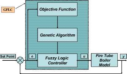
Figure 9. The Structure of GA works on FLC (GFLC)

In this work, our cost function that attempt to optimize the two-control loop, steam/water temperature control loop and water level control loop, keeping the interaction between them, is ISE (Integral of Square Error) for step input over the total simulation time.

t1

ISE = J e2 dt to                                            (3)

Suppose J TOTAL is the overall performance index of the system, which is in the form for a two GFLC controller (four-controller parameter) as shown:

J T = f (C TI , K Tout ) = max (ISE)

J L = f (C LI , K Lou t ) = max (ISE) (4)

where J T is the objective function for temperature controller and C TI , K out is the parameter “C” in the input membership function ,as shown in Fig. 10, and the output-scaling factor respectively for the temperature controller. Also J L is the objective function for level controller and C LI , K Lout are the parameter “C” in the input membership function and the output-scaling factor respectively for level controller, and ISE is Integral of Square Error over the total simulation time.

In order to compatible with the normalization technique, each individual performance index should be dimensionless and represented in term of error for consistency as described below:

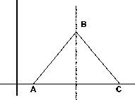
Figure 10 Triangle Membership Function

F T = J T / sum (J T ) F L = J L / sum (J L )

F TOTAL = 1 / (1 + (F T + F L ))        (5)

Where F T is the temperature controller fitness, F L is the level controller fitness and F TOTAL is the overall fitness function of the system. The objective function using fitness produces uniformity from its normalized range [0.1]. In this study, the GFLC controller parameters are given by number of generation = 25, the good convergence was achieved in less than 14 generations. The population size = 100; the structure of the chromosome = [C TI , K Tout , C LI , K Lout ], 4-bit string elements were used for the encoding of each of the four parameters associated with the two GFLC controller, resulting in a total chromosome length of [4 X 4 = 16 bits].

This results in a search space whose size is approximately 65.5X103 points. The method of selection is the roulette wheel method; crossover factor (P x ) = 0.9; mutation factor (P m ) = (0.7/ length of chromosome.

• A. Water/steam temperature control loop

As illustrated previously we attempt to optimize the width of the membership function “Z” and “NOCHANGE” of the input and output membership function respectively and the output-scaling factor at the same time, while leaving other parameters fixed. The parameter “C TI ” was assumed to take values from the interval [5.0, 7.0], for keeping the membership function symmetrical about zero, this will lead to A TI = - C TI for “Z” membership function, C To = 0.006 * C TI , and A To = -C To for “NOCHANGE” membership function. The parameter “K_Tout” was assumed to take values from the interval [2.0, 8.0]. The result in membership functions is shown in Fig. 11.

• b. Water level control loop

As illustrated previously we attempt to optimize the width of the membership function “Z” and “NOCHANGE” of the input and output membership function respectively and the output-scaling factor at the same time, while leaving other parameters fixed. The parameter “C_LI” was assumed to take values from the interval [0.003, 0.01], for keeping the membership function symmetrical about zero, this will lead to A LI = -C LI for “Z” membership function, C Lo = 75 * C LI , and A Lo = - C Lo for “NOCHANGE” membership function. The parameter “K Lout ” was assumed to take values from the interval [2.0, 15.0]. The result in membership functions shown in Fig. 12.

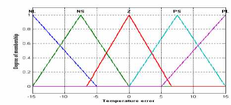
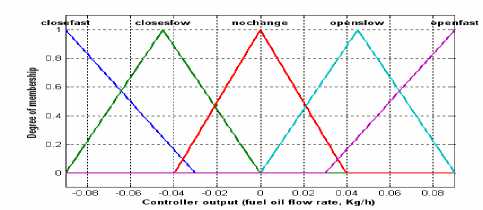
Figure 11. Temperature GFLC membership function

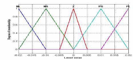
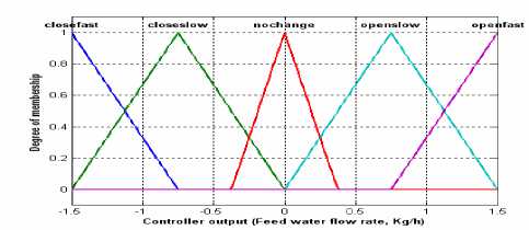
Figure 12. Water level GFLC membership function

maximum oscillation of level is 3.9 mm, reached zero steady state error at 140 sec. With GFLC controller, the level response is oscillatory; the maximum oscillation of level is 0.34 mm, reached zero steady state error at 20 sec. Fig.14, illustrate the variations in water/steam temperature and water level response due to step variation in water level set point (from 0 mm to 20 mm) for fire tube boiler at their nominal capacitance (water content inside shell) with FLC and GFLC controller.

From water/steam temperature response Fig.14-a, shows that, with FLC controller, the temperature response is oscillatory; the maximum oscillation of temperature is 0.14 °C, reached zero steady state error at 132 sec. With GFLC controller, the temperature response is oscillatory; the maximum oscillation of temperature is 0.05 °C, reached zero steady state error at 20 sec. From water level response Fig. 14-b, shows that, With FLC controller, the 2% settling time, ts , is 27 sec with no overshoot and zero steady state error at 98.5 sec. With GFLC controller, the 2% settling time, ts, is 5.4 sec with zero overshoot and reached zero steady state error at 15 sec.

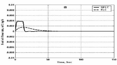
Figures 15-a and 15-b illustrate the water/steam temperature step response of water/steam temperature and water level control variable(output) during the process based on FLC and GFLC controller. Fig.16-a and Fig. 16-b illustrate the water level step response of water/steam temperature and water level control variable(output) respectively during the process based on FLC and GFLC controller.

VI. SIMULATION RESULTS

A MATLAB program is conducted to simulate the dynamics of the plant by using Rung-Kutta fifth order method with tolerance 1x10^-5 .

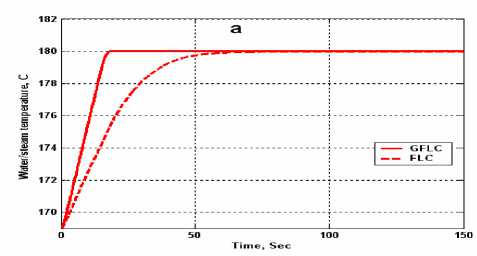
Figure 13, illustrate the variations in water/steam temperature and water level response due to step variation in water/steam set point (from 169 °C to 180 °C) for fire tube boiler at their nominal capacitance (water content inside shell) with FLC and GFLC controller. From water/steam temperature response Fig.13-a, shows that, with FLC controller, the 2% settling time, ts , is 47 sec, with no overshoot and zero steady state error at 80.8 sec. With GFLC controller, the 2% settling time, ts , is 8 sec, the rise time, tr, is 4.5 sec with zero overshoot and reached zero steady state error at 21 sec.

From water level response Fig.13-b, shows that, with FLC controller, the level response is oscillatory; the

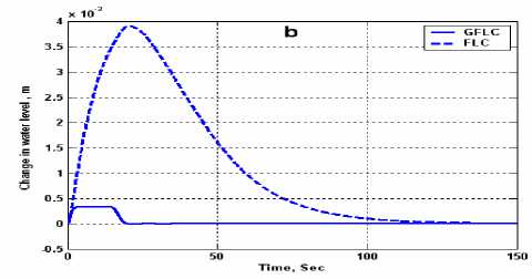
Figure 13. Temperature step response (a) Temperature response (b) Level response

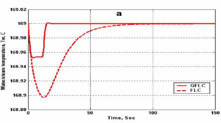
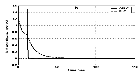
Figure 16. Level step response

(a) Temperature controller output (b) Level controller output

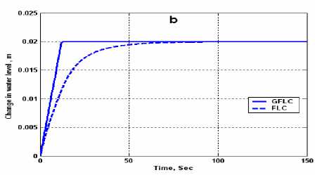
Figure 14. Level step response (a) Temperature response (b) Level response

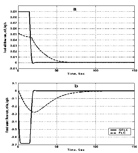
Figure 15. Temperature step response

(a) Temperature controller output (b) Level controller output

VII. CONCLUSION

From the above results and discussion, it can be seen that the fire tube boiler that fitted with GFLC controller has a reliable dynamic performance as compared with the system fitted with traditional FLC controller. Therefore, The GA differs sensationally from more traditional search and optimization method. The four most significant differences are:

• •    GAs searches a population of points in parallel, not a single point.

• •    GAs require only the objective function and corresponding fitness levels, rather than traditional search and optimization method require the derivative information and other auxiliary knowledge; .

• •    GAs based on probabilistic transition rules, not on deterministic rules.

• •    GAs not only works on the parameter but also on the encoding of the parameter itself. (Except in where real – valued individuals are used).