Qualitative features and discontinuous solutions of ideal plasticity equations

This paper examines the qualitative properties and discontinuous solutions of a system of equations of plane ideal plasticity. A continuous homotopy of two classical exact solutions, Prandtl's and Na-dai's, is constructed. It is shown that changing the group parameter leads to a smooth evolution of the characteristics (slip lines), and at a certain value, the characteristics of a single family intersect, leading to the formation of stress discontinuity lines. A qualitative analysis of the characteristic equations allowed us to formulate a sufficient condition for the absence of intersections and, consequently, the continuity of the solution. Using examples of boundary value problems, it is demonstrated that when this condition is violated, the characteristics intersect and discontinuities arise.

Statement of the problem

We consider the system of equations of plane ideal plasticity [1]:

да (   ^'н             о

--2 k cos20— + sin20— l = 0,

дx     l      дx        дy J

да 41    4^    ЭОд0^

2 k sin20--cos20— l = 0,

ду     l     дx        дy J where a is hydrostatic pressure; 0 4 is the angle between the first principal direction of the stress tensor and the axis OX; ks is pure shear yield strength.

We consider two known solutions of the system (1).

Prandtl's solution is often used to describe the compression of a rigid-plastic material by rough plates.

In terms of the variables σ, θ for system (1) this solution has the form

^- P l ^- k s

X l h V

_y 2

— , у = h cos2 0 , h²

where h = const; p ₁ = const.

The boundary conditions will take the form

®| у =± h =- P l - ^x , ⁰| у =± h =ⁿ -                                   (3)

sh

The characteristics of solution (2) are as follows:

x = h (2 0- sin 2 0 ) - h

I A

2 С ⁺ P 1 I ’

I      ks J

y = ± h cos 20, i = 1,2, where ci – const.

Nadai's solution to system (2) describes the plastic state around a circular hole of radius R, loaded with a uniformly distributed normal pressure p ₂ = const and zero shear stress on the hole contour. This solution can be written as

П 0 = ф + 7, 4

CT =

^- P 2 ⁺ k s ⁺ k s ln

x ² + y²

R ²

r ²

= - P 2 + ks ⁺ k s ln—y^ R

where r , φ are polar coordinates.

The boundary conditions take the form

^CT| r = R = P 2 ⁺ k s , ⁰| r = R =^⁺ 4'

The resulting characteristics are as follows:

= 0- 4’

r = R exp ±0 + I

P 2 ^- k s 2 k_s

A + C

J

where c_i – const, i = 3,4.

We construct a homotopy of two exact solutions: Prandtl and Nadai , i.e., a continuous transformation of one solution into the other. This is possible due to the fact that system (1) admits an infinite group of point symmetries; these transformations have the form [2]:

x' = x + ax0(ct,0), y' = y + ay0(ct,0), where (x = x0, y = y0) is arbitrary solution of the system:

d x d0

- 2 k s

cos 20- ^d x + sin 20— I = 0, дст oct J

5 у - 2 k s I sin20* - c«s294 1- 0.

50 I дст         Sct J

We record the solution of Nadai and Prandtl in the following form:

z у    P 2- ks^

x = cos I 0--I Re ² k ^s e^{2 k} s ,

I 4 J

, X    P2-ks JL y = sin I 0--I Re 2 ks e2 ks,

I 4 J hct Ph , • x =1h sin 20, ks    ks(9)

y = h cos2 0 .

We perform a homotopic linear combination of the Prandtl and Nadai solutions:

x = a

^ h ст P i h -- - - -

I k_s k_s

\                 Z X P 2 - ks CT hsin20 +(1 - a)sin 0-— Re 2ks e2ks,

)               (     4 I

z X P 2 - k s _2_ y = ah cos2 0- (1 - a )cos (0- ^П1 Re ^{2 k} s e ^{2 k} s ,

where a is a group parameter.

By analogy with the boundary conditions (6), we seek the boundary curve for solution (10), assuming

n

^ = - P 2 + ks, 0 = T + 4, moving to polar coordinates, we get:

P 2 ~ P 1

r = - 2 ah cos ф + (1 - a )Re ² k s

.

Substituting σ = 2 k_s ( a + θ)into system (10), we obtain parametric equations of the first family of characteristics :

/                           ]              P 2- ks     z x = ah 2(c +0) + P1 + sin20 +(1 - a)Re 2ks cosl 0

Г ' k_s J                (

^^^^^^B

П 1 a +0

4 J e ,

P 2 - ks y = ah cos 20 + (1 - a)Re 2ks

sin ^0--] ea+0

I 4 J

In this case, we can observe the evolution of characteristics that depend on a. For a = 1 , we obtain the characteristics of the Prandtl solution; for a = 0 , we obtain the characteristics of the Nadai solution.

For example, at a value of a≈0.47, the characteristics of the first family intersect (Fig. 1).

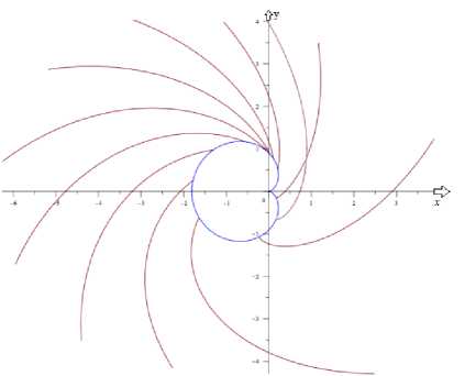
Рис. 1. Пересечение характеристик для отверстия в виде улитки Паскаля a ≈ 0,47

Fig. 1. Intersection of characteristics for a hole in the form of a Pascal snail a ≈ 0.47

Since the characteristics of one family intersect and the values along them are different, the solution of the Cauchy problem cannot be continued continuously after the intersection point. A stress discontinuity line arises. They are considered in [3–7]. This discontinuity line passes along the bisector of the angle [1; 8], formed by intersecting characteristics, and emerges from the point of their intersection.

Figure 2 shows a stress discontinuity line. Next, we'll explore the conditions under which it occurs.

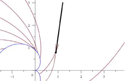
Рис. 2. Линия разрыва напряжений

Fig. 2. Stress discontinuity line

Discontinuous solutions of the Cauchy problem

Cauchy problem (initial value problem). A smooth arc is defined in the x, y plane, nowhere coinciding with the characteristic directions and intersected by each characteristic only once, where x = x ( s ), y = y ( s ), s , and s is a certain parameter. The functions σ(x, y), θ(x, y) are defined along L.

To find the conditions for the occurrence of discontinuities, we will conduct a qualitative study. From system (1), by replacing

σ=ks(ξ+η),θ= 12(η-ξ)

we obtain

∂ξ+∂ξtgθ=0,

∂ x ∂ y

∂η ∂η

• -    ctg θ = 0.

∂ x ∂ y

We consider the first equation (12), it has two integrals:

dx dy  d ξ

1 = tgθ = 0 , dy = tgθ, ξ = ξ0 = const. dx dy

For a qualitative study of the solution of the equation    = tgθ we represent its solution in the form dx y=tgθx+ ψ(θ),                                     (14)

where ψ(θ) is a n arbitrary function.

Let this solution satisfy the boundary condition

^{θ = θ} 0 ^{( x )} where y = 0.

We consider two solutions (characteristics) of the form (14), passing through the points ( x 1 ,0) and

( x 2 ,0) (Fig. 3), from (14) we have:

y=(x-x1)tgθ1, θ1 =θ(x1), y=(x-x2)tgθ2,θ2 =θ(x2).

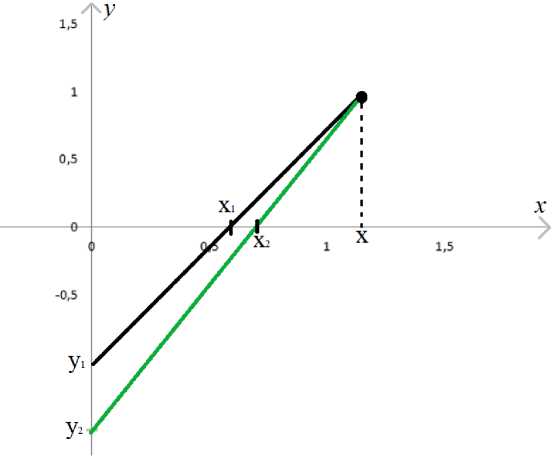
Рис. 3. Пересечение характеристик одного семейства

• Fig. 3.    Intersection of characteristics of one family

We find the intersection point of these characteristics:

У 2 - y 1 x                   .

tg ⁹ 1 - tg 0 2

Since ^y i >  ^y 2 , ^tg ^ i <  ^{tg 9} 2 , тогда 9 1 <0 2 , therefore , the function ^{9 (} x ) increases. Thus, a qualitative study provides the following conditions for the intersection of characteristics of one family:

For the intersection of characteristics along which ^e = const , it is enough that ⁹ = ⁹ o ⁽ x ) is an increasing function.

We check these conditions using numerical-analytical solutions.

Calculating characteristics using conservation laws

In the works [2; 10–12] a method for solving the Cauchy problem based on the conservation laws of the original plasticity system was proposed.

We are looking for conservation laws for system (1) in the form of functions C = C(σ, θ),

D = D(σ, θ), for which the equality	д С d D n &=0                                (15)
is reduced to the form	дD д C n n — - —tg 9 = 0,                            (16) де   de, дD д C  n n —+ —ctg 9 = 0.                           (17) дп дп

Introducing new dependent functions φ, ѱ,

ф = D - tg0 C, V = D + ctg9 C,                                (18) we obtain the system

∂ϕ 1

- tg θ ( ψ -ϕ ) = 0,

∂ξ 2

∂ϕ 1

+ ctgθ(ψ - ϕ) = 0.

∂η 2

After replacing variables according to the formula ^{ρ =ϕ cos θ} , we arrive at the equation

ρ

^ρ ξη ^- ₄ ^{= 0,}                                        (20)

i.e. to the well-known telegraph equation.

We record the integral over the closed contour SPR. Here SP is the boundary curve; RS are the characteristics of the first family; RP are the characteristics of the second; R is the intersection point of the characteristics. Using relation (15) in Stokes' theorem for the plane [13], we conclude that this integral is equal to zero:

J Ddx — Cdy = J + J + J = 0-

SPR               SP PR : η=η ₀ RS : ξ=ξ ₀

For the coordinate у_R ,, assuming φ = 1, ѱ = 0, we obtain boundary conditions for system (19) of the form

ϕ _RS = 1, ψ _PR = 0.                                       (₂₁)

Under these conditions, the expression for the coordinate xR takes the form xR = ∫ (Ddx-Cdy)+xs.

_SP                                                      (22)

Similarly, for the coordinate у R , sloping φ = tgθ, ѱ = 0, we obtain boundary conditions for system (19) of the form

ϕ _RS = tg

^{η -} ₀ ^{ξ 0} , ψ PR = 0.

Under these conditions, the expression for the coordinate y R takes the form y_R = ∫ ( Ddx - Cdy ) + y_s .

SP

Considering that φ, ѱ are related to the function ρ as follows :

ρ 2 ∂ρ

ϕ= , ψ= cos θ      sin θ ∂ξ ,

we get two problems:

∂ ² ρ _- ρ _{= 0,}

∂ξ∂η 4

^ρ ξ=ξ 0 ⁼

η-ξ cos ⁰ , 2

∂ρ ∂ξ

= 0.

η=η ₀

∂2ρ -ρ=0, ∂ξ∂η 4

ρ

ξ=ξ 0

= sin

η-ξ ₀ 2

∂ρ

= 0.

The solution to problem (26) for the coordinate x_R is the function

ρ=ρ1(ξ,η)=I0(4(ξ-ξ0)(η-η0))cosη02-ξ0 - 12 ∫I0(л/(ξ-ξ0)(η-τ))sinτ-2ξ0 dτ,

η ₀

along with this

^{∂ρ 1} = ¹cos ^{η 0 -ξ 0} I 1 ( 7 ( ξ-ξ ₀)( η-η ₀) η-η 0 _- 1 _∫ ^η _{I 1(}7( ξ-ξ ₀)( η-τ )) ^η-τ sin ^{τ-ξ 0} d τ .

∂ξ 2       2    1        0       0 ξ - ξ 4   1        0          ξ - ξ 2

The solution to problem (27) for the coordinate y R is the function:

ρ=ρ2(ξ,η)=I0( (ξ-ξ0)(η-η0))sinη02-ξ0 - 12 ∫ηI0( (ξ-ξ0)(η-τ))cosτ-2ξ0dτ,

η ₀

along with this

^∂ρ ² = ¹sin ^{η 0 -ξ 0} I 1 (7( ξ-ξ 0 )( η-η 0 ) ^{η-η 0} + ^{1 η} ∫ I 1 (7( ξ-ξ ₀)( η-τ )) η^-τ cos ^{τ-ξ 0} d τ ,

∂ξ 2      2    1        0       0 ξ - ξ 4   1        0          ξ - ξ 2

where I ₀ is is a Bessel function of the first type of imaginary argument.

T he functions φ, ѱ are reconstructed using formulae (25). The components of the conservation laws are determined from relations (18):

D =ψ sin² θ+ϕ cos² θ , C = ( ψ - ϕ ) sin θ cos θ .

We find the coordinates of point R by substituting the found C and D into formulas (22) and (24).

Calculations of characteristics for known exact solutions

We construct characteristics for equations (1) using the method described in the previous section. To construct characteristics of the Cauchy problem for ideal plasticity equations using conservation laws, we developed programs in the Maple environment [14; 15]. To test the program, we constructed known characteristics of the Pradtl and Nadai solutions.

Having tested the program on these two solutions, it was concluded that it produces relevant solutions. The calculation error is of the order of 10–8.

Construction of discontinuous solutions

To verify the non-intersection condition of characteristics of a single family, characteristics with different boundary conditions were constructed. Let's consider some of them. We set the following boundary condition. Using the program, we constructed two characteristics of the first family until they intersected. The result is shown in Figure 4.

σI _{y = 0} =σ ₀( x ) =- x + 1, θ

_{y = 0} =θ ₀( x ) = x - π ₄.

For the boundary value problem (33), the condition that the function θ is non-increasing is violated, and a discontinuity in the solution occurs.

We set the following boundary condition. Using the program, we plot two characteristics of the first family up to their intersection. The result is shown in Figure 5.

σ I _{y = 0} =σ ₀( x ) = 1, θ I _{y = 0} =θ ₀( x ) = x ².

In the case of the boundary value problem (34), the condition of non-increasing function θ is violated and a discontinuity in the solution arises.

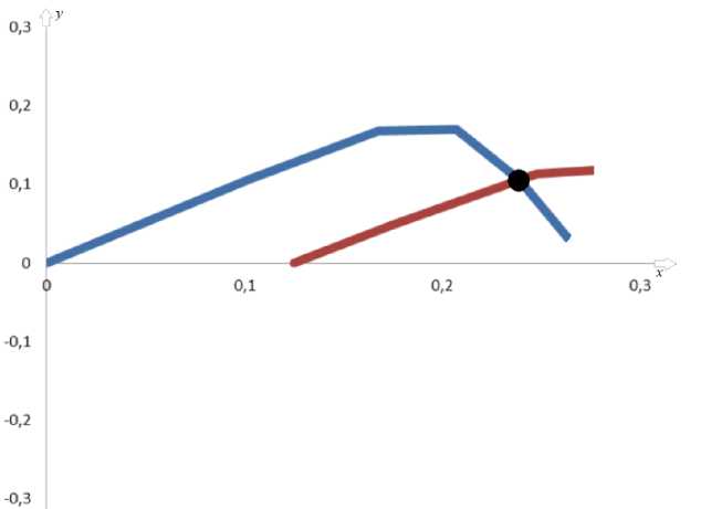
Рис. 4. Пересечение характеристик первого семейства при граничном условии (33)

• Fig. 4.    Intersection of the characteristics of the first family under the boundary condition (33)

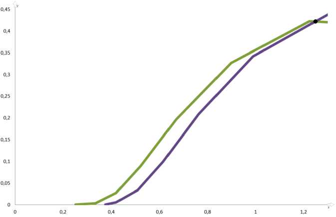
Рис. 5. Пересечение характеристик первого семейства при граничном условии (34)

Fig. 5. Intersection of the characteristics of the first family under the boundary condition (34)

Conclusion

Thus, it is shown that the Cauchy problem does not have a continuous solution for all boundary conditions, but a qualitative study and numerical-analytical calculation gives the following condition for the continuity of solutions: for the continuity of the solution of the Cauchy problem, it is sufficient that ® = $ o ( x ) is a decreasing function.

Работа поддержана Красноярским математическим центром, финансируемым Минобрнауки РФ (Соглашение №075-02-2026-1314).

Acknowledgements

This work is supported by the Krasnoyarsk Mathematical Center and financed by the Ministry of Science and Higher Education of the Russian Federation (Agreement №075-02-2026-1314).