Rate of Convergence of the Sine Imprecise Functions

Published Online October 2016 in MECS

Imprecise function which is obtained by the multiplication of some other functions is called multiplication factor. Thus any continuous function is multiplied by sine or cosine function to obtain imprecise polynomials. For a certain region we will collect finite number of data collection of points. And with the help of these points we will identify most valuable function or the controllable function called imprecise function for these points.

Area bounded by the imprecise function help us to know how the variation of the effect of impreciseness of an object is occurred for the different intervals. For this reason we define formula of the area of an imprecise number in the general summation form. Thus the area formulae of the different angles of sine functions are also play an important role in this article.

The remaining sections of the article are divided into the following ways:

Section II is contain about the preliminary definition of imprecise function, section III is contain definition of new function called imprecise function, Section IV is contain conversion point obtain by the help of multiplication of the sine and cosine function, Section V is contain rate of convergence of different imprecise function so that we can study variation of the effect of imprecise for the respective intervals. Finally section VI is the conclusion and the summary of this article.

• II.    P reliminaries

Before starting this article it is necessary to recall the definition of imprecise number, partial presence, membership value etc. over the real line which are discussed in the article [9],[10],[12] [13], [15] and [16].

• A.    Imprecise Number:

Imprecise number is a closed interval N=[α,β,γ] which is divided into closed sub-intervals with the partial presence of element β in both the intervals.

• B.    Partial presence:

Partial presence of an element in an imprecise real number [a, p, у] is described by the present level indicator function p(x) which is counted from the reference function r(x) such that present level indicator for any x, a <  x < у , is (p(x) — r(x)) , where 0 <  r(x) <  p (x) < 1

• C.    Membership value:

If an imprecise number N = [а,Р,у] is associated with a presence level indicator function ^(x) such that,

(цi (x),   when a < < P P p2 (x),   when X X x < у

0,        h

With a constant reference function 0 in the entire real line. Where ( ) is continuous and non-decreasing in the interval [ ,  ] , and ( ) is a continuous and nonincreasing in the interval [ , ] with цi (a) = ц 2 (У) = 0, then (  ( ) —   ( )) is called membership value of the indicator function ( )

• D.    Normal Imprecise Number:

A normal imprecise number N = [a, p, у] is associated with a presence level indicator function ( ) such that,

(цi (x),      hhen a < x < P ц2 (x),     when P < x < у

0,                 h

With a constant reference function 0 in the entire real line. Where ц(x1) is continuous and non-decreasing in the interval [ , ] and ( ) is a continuous and nonincreasing in the interval [ , ] with ц i (a) = ц ((у) = 0

ц i (Р) = ц (СР ) = 1

Here, the imprecise number is characterized by {х, ц ^ (х), 0 : х е R } , R being the real line.

For any real line, 0 < цi (x) < ц( (x) < 1 normal and subnormal imprecise number will be characterized in common, {x^ 1(х),ц2(%): x е R }, where цi(x) is called membership function measured from the reference function ( ) and (  ( ) —    ( )) is called the membership value of the indicator function.

Here, the number is normal imprecise number when membership value of indicator function ц_м (x) is equal to 1 otherwise subnormal if not equal to 1. Moreover if the membership value of ц_м (x) is equal to 1 then the set is universal set and the null or empty set if the value of p_N (x) is equal to 0.

• III.    I mprecise F unctions

Imprecise number is an interval definable number where the interval is an area bounded by some section of a function formed by the impreciseness of objects. So, the function which contains such type of imprecise intervals within in it is known imprecise function. At present this phenomenon is occurring available in the field of science and technology. For example possible of impreciseness of electromagnetic wave frequency in between the server and the receiver is an imprecise function. Where, the finite numbers of imprecise numbers are occurred in between the locations. So, the bigger function to connect these two locations is an imprecise function. From this point of view it can be introduced some conditions for the imprecise functions as follows:

• (i)    Function must be continuous in some region

• (ii)    Function should be oscillation in nature

• (iii)    Function must have finite number of maximum and minimum values within the interval.

• (iv)    Function should be semi-periodic/periodic in nature.

Generally, formation of effect of the impreciseness in the form of sine and cosine functions for a certain region is interval definable number. Thus, effect of any function which is defined for any intervals can be converted into imprecise function with the help of multiplication factors of sine and cosine functions.

• A. Conversion point-

• It is a point from where non- imprecise function starts to convert into imprecise function. If we can identify this point, then we will get easily their applications. As for example loudness of sound causes brain and heart diseases because of non-imprecise function of character produces from a sound device. So, it may be possible to control by converting them into human ear audible level by the help of volume regulatory. Further in present most of the times ultraviolet ray reaches in the ground is non-imprecise function form due to lake of the friction of Ozone layer caused by the environmental pollutions. This phenomenon is creating problems in the life of living being causing skin disease etc. Thus if we can invent a new device having Ozone layer character, then it will save us from these type of problems. This may be possible due to the multiplication factor which can convert any function into imprecise function form.

Normally these phenomena are already applied in many of the experiment like volume regulator or the regulators used in the different fields for their practical purposes.

• IV.    C onversion of P olynomials into I mprecise F unctions

There are many polynomials, which are raised to infinite direction without coming back to the ground level. So it is called uncontrolled function. But this type of function can also be transformed into oscillation form to meet the ground level repeatedly from a certain point. This point is known as conversion point. This phenomenon is occurred by the multiplication of a function which can convert into imprecise function form. This multipliable function is called multiplication factors.

Thus the imprecise function obtained by the multiplication of sine function is known as sine imprecise function and the imprecise function obtained by the multiplication of cosine is called cosine imprecise function.

For this purpose, let us consider

Pl (Х1 , У1 ), Р2 (Х2 , У2), Рз (хз , Уз)……………․․ ……………․Рп (%п+1, Уп+1), be the nth collection of points, which are above and below the given polynomial of degree n,

• У =  + с_±х + с₂х² + с₃х³ ……․․+ с_пх      (1)

To convert it into imprecise form, let us multiply this polynomial by a sine function.

Thus,

У =(Со + с_гх + с₂х² + с₃х³ + ………․․+ с_пх ) sin( 1х ); leZ         (2)

will be a sine imprecise polynomial of degree n.

To obtain standard imprecise polynomial averagely passing closed to these points, we follow the rules of matrix multiplication as follows:

As, the point Pl , р₂ ,………………․ Рп are satisfied the given polynomial. By the law of roots, we will get n^th set of simultaneous linear equations having arbitrary constants С₀, Ci ,С 2 ,………………․․

․․……,c_n as follows:

У1 =(^со + С1^Х1 + c₂Xi² + Сз^х1³ ………………………+ Си ^-1 )sin( 1х_т )

У2 =(^со + С1Х₂ + С₂^Х₂ + Сз^х2³ ………………………+ Си ^2 )sin( 1х₂ )

Уз =(^со + С1^хз + с₂х₃² + Сз^хз³ ………………………+ Си Х₃ )sin( 1х₃ )

Уп=(со + Ci%n + С2ХП2 + Сзхп3 ………………………+спхп ) sin(^)

Which can be written in the matrix form as гУ.]

⎢⎡⎥

⎣⎦

[ ( 1х_А ) х_г sin( lx_t ) sin ( lx₂ ) ^х2 sin( lx₂ )

sin ( lx_n ) Xn sin( lx_n )

x-^sin ( lx_t ) x₂ⁿsin ( lx₂ )

x_nⁿsin ( lx_n )

]

ГСО] ⎢⎡ 2 ⎥⎤

⎣

≅    =   ( say )

Where,

A = ⎢ 1

2      3     4                 /у П

1  Ai   Ai  Ai …………․  Ai I x2 X22  x23 x24  …………  ^2” ⎥

…………

To obtained the solutions of arbitrary constants, we write,

AT (AX)=ATB(6)

Where A^T is the transpose matrix of A.

Values of ATA = ( aH )

(     )×( ti+ 1.)

and ATB = (bt)(n+1)×1

such that aij =∑k=l[xk’"2{sin(lxk )}2 ]

and bi =∑ k=l [ Ук^хк sin( lx_k )],1 ≤ i ≤( n +1) (10)

n= order of the polynomial, m=no of collection of points, Xt and 7t ordinates and the abscissa of the given points.

Solution     of     the     arbitrary     constants

Cq , Cl , c₂,………………………,c_n can be obtained with the help of Gauss-elimination method of general form

Rt → Ri -          × at, ;

a ( i-l )( i-l )

(2≤ i ≤n+1),(1≤ j ≤n)

Steps of transformation will be done as follows:

(2≤ i ≤n+1wℎen j =1)

(3 ≤ i ≤и+1wℎen j =2)

(и+1≤ i ≤и+1wℎen j = )      (11)

These operations help us to get upper triangular matrix. By backward substitution we will get the solution of the mentioned arbitrary constants.

Thus any polynomial can be obtained into controllable form by multiplication of sine and cosine function.

For the different value of I we will get different value of the constants. Because of different value of the constants we will have different imprecise functions. This characteristic of function is very important in the field of applications.

A. Sine imprecise Polynomial of degree one-

Example-1 ( Sine imprecise function of polynomial of degree one with angle, X):

Let У=   + c4x be a polynomial of degree one. So, in particular

У =(Со + с₄х ) sin( X ), for I = 1       (12)

is a sine imprecise polynomial of degree one.

Let us consider     (1,3.2),   (2,4),(3,-2.5),   (4,

• 4.5) ,(5,6),(6,-7.5),(7,5.5) be the points in the data collection which are above and below the x-axis.

So, %! =1,Х₂ =2,х₃ =3,х₄ = 4, х₅ =5,х₆ =6,X?=7

У1 = 3․2, Уг =4,Уз = -2․5,

У4 = -4․5, Уз =6,Уб = -7․5, У? = 5․5

By the law of roots the given imprecise function satisfies the given collection of points to have linear simultaneous equation to form a matrix as follows:

From (4), (5), (6) …………․․․ (10), we have

АХ =

=>( А^ТА ) X =

Where, А^ТА = ( ан ) ^,               ₍п+1)×(п+1)

ЛЧ = ( ац )₍ п+1)× 1 ^,х=* +

Such that Оц =∑ ™=1^хк ⁷   {sin( Х_к )}²

and Ь[ =∑ ™=1УкХк sin( Х_к ), 1 ≤ i ≤( п +1)

Here, m=no. of points=7, n= degree of the polynomial=1

А^ТА = ( ац ) _{2 х 2} and А^ТВ = ( bi )2 ×1

Where Clij =∑ k=l^xk ⁷ {sin( Х_к )}²

and bi =∑ к=1Ук^хк sin( ^хк ), 1 ≤ i ≤2

=∑ {sin( )} 2 ац =∑хк {sin(хк )} к=1

=    ( Х1 )+ sin² ( х₂ )+ sin² ( х₃ )+ sin² ( х₄ )

+ sin² ( ^5)+ sin² ( х₆ )+ sin² ( х₇ )

= 0․04250,

=   =∑  {sin( )} ,

=   =∑  {sin( )} к=1

=      ( х_г )+ x₂sin² ( Х₂ )+ x₃sin² ( х₃ )+ x₄sin² ( х₄ )

+ x₅sin² ( х₅ )+ x₆sin² ( х₆ )

+ x₇sin² ( х₇ )

= 0․23883

«22 =∑ ^Хк² {sin( Хк )}²

к=1

=       ( Х1 )+ x₂²sin² ( х₂ )+ x₃²sin² ( хз )

+ x₄²sin² (х₄)+ x₅²sin² ( ^5 ) + x₆²sin² ( х₆ )+ x₇²sin² ( х₇ )

= 1․141868, bi =∑УкХк sin(хк )

к=1

=     sin( Х1 )+ УгХ₂ sin( х₂ )+ УзХз sin( Хз )

+ у₄х₄ sin( Хд, )+ У5Х5 sin(%5 )

⁺ У₆х₆ sin( Хб )+ у₇х₇ sin( х? )

= 1․345599

=∑    „п(, )

°2 =∑ Ук^хк sin( )

к=1

=      sin( Х1 )+ У₂х₂ sin( х₂ )+ УзХз² sin( Хз )

+ у4х42 sin(%4)+У5^52 sin(%5 )

⁺ Уб^б² sin( Хь )+ у₇х₇² sin( х₇ ) = 12․10867

0․04  0․23 Со     1․34

^{Thus *}0․23   1․41^{+ *}С1^{+ = *}12^․․10⁺

From the formula (11), we have

^ → Ri -         _× ац ; (2 ≤ i ≤ 2), (1 ≤ j ≤1)

Cl ( i-i )( t-г )

0․04   0․23  со+=*1․28+

0    0․087 ci + = *4․39+

=> 0․04с0 + 0․23С1 = 1․28, 0․087С1 = 4․39

So, ^ci =   ^․ 39 = 50․45,

1    о․087

с0 =004(1․28-0․23ci )

0․04

=     (1․28 - 0․23 × 50․45) = -258․08

0․04

So, У = (-258․08 + 50․45 х ) sin( х )          (13)

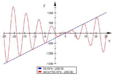
Fig.1. Graph of y = -258․08 + 50․45x and y = (-258․08 + 50․45x)sin(x)

Here, 258 ^․ 08 = 5․115 QTld к < 5․115 < 2 It , for which ,                ․                               ^{․                                                                  ․                                           ,}

X=       2и are the nearest two values such that sin(X)=0

So, the graph starts to oscillate from the point, X = ․       ≃ 5․699( approx․ ) along the positive x- axis and X = ․     ≃ 4․128(approx)․ along the negative x-axis which is shown in the Fig1.

So,

5․115 + 2 n                    5․115 + 2 n      5․115 + 2 П \

.           , (-258․08 + 50․45 (          )) sin(          )/

Such that ац =∑ k'=l^xk ⁷ {sin(2 X_k )}² and = ^∑ к=1Ук^хк sin(2 ^xk ), 1 ≤ i ≤( П +1)

Here, m=no. polynomial=1

of points=7 and n= degree of the

A^TA = ( ^aij )

V      ×2

and A^TB = ( а_ц )

V      ×1

Where CLij =∑ k=l^xk ⁷ {sin(2 ^xk )}² and = ^∑ к=1Ук^хк sin(2 ^xk ), 1 ≤ i≤2

dll =∑ ^xk° {sin(2 ^xk )}²

k=l

=    (2%1)+ sin² (2 ^X2 )+ sin² (2 ^X3 )+ sin² (2 x₄ )

+ sin² (2 ^xs )+ sin² (2 ^x6 )+ sin² (2 ^xi )

= 0․16828,

«12 =    =∑ ^Xk {sin(2 ^xk )}²

k=l

=      (2 X1 )+ x₂sin² (2 X₂ )+ x₃sin² (2 x₃ )

+ x₄sin² (2 x₄ )+ x₅sin² (2 ^x5 ) + x₆sin² (2 x₆ )+ x₇sin² (2 x₇ )

= 0․94102, is called conversion point along the positive x-axis.

Example-2 (Sine imprecise function of polynomial of degree one with angle, 2 X):

Let У=   + сгх be a polynomial of degree one. So, in particular

У =(Co + с_гх ) sin(2 X ), for I = 2        (14)

is an imprecise polynomial of degree one.

Let us consider the same example taken for the equation (12)

Here,      (1,3.2),      (2,4),(3,-2.5),(4,-4.5),(5,6),(6,-

• 7.5) ,(7,5.5)are the points in the data collection which are above and below the x-axis.

a-22 =∑ ^xk² {sin(2 ^xk )}²

k=l

=       (2%1)+ x₂²sin² (2 ^X2 )+ x₃²sin² (2 ^X3 )

+ x₄²sin² (2 x₄ )+ x₅²sin² (2 ^xs ) + x₆²sin² (2^x&)+ x₇²sin² (2 ^xi )

= 5․60673, bl =∑Укхк sin(4)

k=l

=     sin(2 ^X1 )+ У2^Х2 sin(2 ^X2 )+Уз^з sin(2 ^X3 )

+ У4Х4 sin(2X4)+У5^5 sin(2Xg )

+ Уб^б sin(2%5)+ У?^Х7 sin(2X? )

= 2․49223

So, ^X1 = 1, x₂ = 2, x₃ = 3, x₄ = 4, x₅ = 5, x₆ = 6, x₇ =7

У1 = 3․2, y2 = 4, Уз = -2․5,

У4 = -4․5, Уб = 6, Уб = -7․5, У? = 5․5

By the law of roots the given imprecise function satisfies the given collection of points to have linear simultaneous equation to form a matrix as follows:

From (4),(5),(6)………….(10),we have

AX =

=> ( A^TA ) X =

Where, ДТД = ( ^ач )₍ n+1)×(n+1)

ATB = (bt)(n+1)×1,X=*Cl + b2 =∑Укхк2 sin(4)

k=l

=      sin(2 ^X1 )+ У2^Х2² sin(2 ^X2 )+ Уз^хз² sin(2 ^X3 )

+ У₄^Х4² sin(2X4)+ У5^Х5² sin(2Xg )

+ Уб^б2 sin(2Xg)+У7Х72 sin(2X?)

= 23․96444

0․16  0․94 co     2․49

^{Thus *}0․94  5․60^{+ *}Cl^{+ = *}23^․․96⁺

From the formula (11),we have-

^Rt → ^Rt ^-

Rj

^{× a}tj ^; a ⁽ t-i )( t-i ⁾

(2 ≤ i ≤ 2), (1 ≤ j ≤ 1)

0․16 0․94 co+=*2․49+ 0    0․07 Cl + = *9․33+

So, as above we get

У4 = -4․5, Ув =6,Уб = -7․5, У? =5․5

=> 0․16с0 + 0․94С1 = 2․49,    0․07С1 = 9․33

9․33

С =90․․3037=133․28,

Со =     (2․49 - 0․94С1 )

0․16

=     (2․49 - 0․94 × 133․28) = -746․64

0․16

So, У = (-746․64 + 133․28 х ) sin(2 х )     (15)

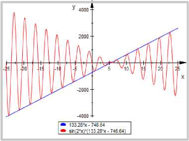
Fig.2. Graph of = (-746․64 + 133․28x) and y= (-746․64 + 133․28x)sin(2x)

Here, ․  ≃ 5․60 and —<5․60<2и for which X=        2л are the nearest two values such that sin(2X)=0

So, the graph starts to oscillate from the point, X = ^․ 60+27Г ≃ 5․9423( approx ․) along the positive x-axis and х = ^× - ^․ 60+Зтг ≃ 5․156( approx ․) along the negative x-axis which is shown in the Fig 2.

So,

-746․64 +

․ 60+2лЛ 1

5 ․ 60+27ГА ×sin(2× ․ ₎

133․28 (      )

By the law of roots the given imprecise function satisfies the given collection of points to have linear simultaneous equation to form a matrix as follows:

From (4),(5),(6)………….(10),we have

АХ =

=>( А^ТА ) X =

Where, л^гл = ( ац )₍ п+1)×(п+1)

А^ТВ = ( b_t ) ₍ п+1 )× 1, X =*С1 +

Such that ^aij =∑ ™=1Хк ⁷ {sin(3 Х_к )}² and = ^∑ к=1Ук^х_к sin(3 ^хк ), 1 ≤ i≤(п+1)

Here, m=no. of points=7 and n= degree of the polynomial=1

АТА = ( ац ⁾₂×₂ and А^ТВ = ( ац ⁾₂× .

Where aij =∑ к=1^хк ⁷ {sin(3 ^хк )}² and = ^∑к=1Ук4sin(3 ^хк ),1 ≤ i ≤2

∑

^хк° {sin(3 ^хк )}²

к=1

=    (3%1)+sin² (3х₂)+sin² (3 ^хз )+ sin² (3 х₄ )

+ sin² (3 ^х5 )+ sin² (3 х₆ )+ sin² (3 х₇ )

= 0․27677,

∑ ^Хк {sin(3 ^хк )}² к=1

а12 =

=       (3_Х1)+ x₂²sin² (3 ^Х2 )

+ x₃²sin² (3 ^хз )+ x₄²sin² (3 х₄ )

+ x₅²sin² (3 ^xs )+ x₆²sin² (3 ^х& ) + x₇²sin² (3 ^xi )

= 2․077794, is called conversion point along the positive x-axis.

Example-3 (Sine imprecise function of polynomial of degree one with angle, 3 X):

Let У=   + с^х be a polynomial of degree one. So, in particular

У =(Со + с^х ) sin(3 X ), for I =3       (16)

∑ ^хк² {sin(3 ^Хк )}²

к=1

x^sin² (3_Х1)+ x₂²sin² (3 ^Х2 )+ x₃²sin² (3 хз )

+ x₄²sin² (3 х₄ )+ x₅²sin² (3 ^5 ) + x₆²sin² (3 х₆ )+ x₇²sin² (3 %₇ )

= 12․36365, is an imprecise polynomial of degree one.

Let us consider the same example for the equation (12)

Here, (1,3.2),(2,4),(3,-2.5),(4,-4.5),(5,6),(6,-7.5),(7,5.5) are the points in the data collection which are above and below the x-axis.

So, х_г =1, х₂ =2, х₃ =3, х₄ =4, х₅ =5, х₆ =6, х₇ =7

У1 = 3․2, У2 =4,Уз = -2․5,

∑ УкХ_к sin(3 х_к )

к=1

=     sin(3 Х1 )+У 2X2 sin(3 Х2. )+ У 3X3 sin(3 Хз )

+ у₄%4 sin(3%4)+ У5Х5 sin(3 ^XS )

+ У&х₆ sin(3 ^Х6 )+ у₇х₇ sin(3 X? )

= 3․744006

=∑     sin(3xk)

=∑     sin(3 )

k=l

=     sin(%1)+Уз^ sin(3^2)+Уз^з2 sin(3X3 )

+ У4Х42 sin(3X4)+У5^52 sin(3Xg )

+ Уб^б2 sin(3Xg)+У7%72 sin(3X? )

= 35․319439

0․27   2․07   co1 _

^{Thus *}2․07 12․36^+*Cl+=

3․74

*35․31+

From the formula (11),we have-

^Ri → ^Ri ^-

Rj

×

a ( t-i )( t-i )

^ij ^;

(2≤ i ≤2),(1≤ j ≤1)

0․27

*0

2․07  co+=*3․74+

3․51 Cl+ = *6․63+

-

So, as above we get

=> 0․27 Co + 2․07Cl=3․74,-3․51Cl = 6․63

6․63

Cl =  ․    =-1․888,

-3․51

co =027(3․74-2․07ci ) 0․27

=     (3․74 - 2․07 × (-1․88))

0․27

= 28․26

So, У =(28․26-1․88 x ) sin(3 x )         (17)

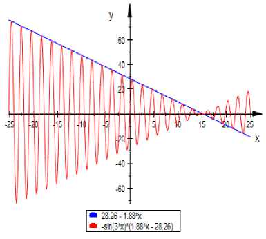
Fig. 3. Graph of y = (28․26 - 1․88x) and y = (28․26 - 1․88x)sin(3x)

Here, ^․   ≃ 15․03( approx ․)   QTld —<15․03<

1 ․88               x             ✓              3

5 я , for which X =         5я are the nearest two

з values such that sin(3X)=0

So, the graph starts to oscillate from the point, X=  ․ 03+5тг ≃ 15․370(approx․) along the positive x- axis, and x= × - ․ 03 + 1471 ≃ 14․837(approx․) along the

negative x-axis which is shown in the Fig 3. So,

( ․ 03 + 5тг no       1 oor15 ․ 03+57ГXX .        15 ․ 03+57Гх \

․      , (28․26 - 1․88( ․     ))sin(3 ×  ․     ))m is called conversion point along the positive x-axis.

B. Sine imprecise function of polynomial of degree two:

Let у=   + сгх + c±x2 be a polynomial of degree two. So, in particular

У =( Cq + с_гх + C₁X² ) sin( X ), for I =1     (18)

is an imprecise polynomial of degree two.

Let us consider (1,0.5), (2,2.5),(3,2),(4,4),

(5,3.5),(6,6),(7,7) be the points in the data collection.

So, %1=1, ^2 =2, ^3 =3, X₄=4, ^5 =5, ^6 =6,X?=7

У1 = 0․5, У2 = 2․5, Уз =2,

У4 =4,У5 = 3․5, Уб=6,У? =5․5

From (4),(5),(6)………….(10),we have

AX =

=>( A^TA ) X =

Where A^TA = (^a7/)

( 71+1)×(    )

and A^TB = ( bn )₍n+1)×1

Such that ^aij =∑ ™=l^xk ⁷   {sin(X_k)}²    and ⁼

^∑ к¹=1Ук^хк sin( ^xk ), 1 ≤ i≤( П +1)

Here, m=no. of points=7 and n= degree of the polynomial=2

A^TA = ( Clij ⁾₃×₃ and ATB = ( dtj ⁾₃×4

Where at] =∑ k=l^xk ⁷ {sin( ^xk )}² and bi =∑ к=1Ук^хк sin( ^xk ),1 ≤ i ≤3

∑ ^xk° {sin( ^xk )}²

k=l

= 0․0148521,

a13

=

∑ ^xk {sin( ^ )}² k=l

= 0․341889,

∑[ ^xk² {sin( ^xk )}²]

k=l

=∑ ^xk {sin( ^xk )}²

k=l

= 1․418684

= 0․341889,

And

Thus

Я₂₂ =∑ X_k² {sin( X_k )}² = 1․1418684, k=l

a32 =∑Xk3 {sin(xk)}2 = 8․799282, k=l a33 =∑Xk4 {sin(Xk)}2 = 56․055255 k=l

bl

=∑ X_ky_k sin( X_k ) = 11․593562,

k=l

^2 =∑хк2Укsin(Xk) = 68․812246, k=l

Ь₃ =∑ х_к³Ук sin( Xk ) = 424․896557

k=l the simultaneous equation is converted

into

461․55c2 = 5143․86

So, ^co = -78․13, ^C1 = 0․63, c₂ = 11․14 and = (-78․13 + 0․63 x + 11․14 x² )sin( X )        (19)

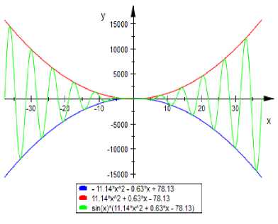
Fig.4. 2D graph of y = (-78․13 + 0․63x + 11․14x )sin(x)

Thus the solution is

0․63 ± √0․63 +4×78․13×11․14

=           2×78․13

= 0․38( approx ),-0․37( approx ) and - я <-0․37<0 and 0< X < H

following simple matrix form:

0․015

[ 0․34

1․14

0․34

1․14

8․80

1․14 1 [C°      11․59

8․80][Cl]=[68․81] 56․06J Lei     424․90

From the formula (11),we have-

Ri → Ri -            × O-ij ; ci (i-l)(i-l)

0․015

(2≤ i ≤3); j =1

0․34

-6․56

-17․04

11․59

1․14

-17․04

-30․58

][ « ]

-193․89

-455․94

R[ → Ri -            × O-ij ;

Cl ( i-l )( i-l )

(2≤ i ≤3); j =2

0․015   0․34     1․14	co"		11․59
[  0    -6․59  -17․04]	[Cl	=	-193․8]
0       0     461․55	A.		5143․86

=> 0․015c0 + 0․34Cl + 1․14c2 = 11․59

=> -6․59Cl - 17․04c2 = -193․98

So, the graph starts to oscillate from the point, X= ․    ≃1․76(approx) along the positive x-axis, and X =  ․    ≃ -1․75( approx) along the negative x-axis which is shown in the Fig 4.

So,

₍ °- ^․ 38+.,(-78․13+0․63( “ ^․ 38+.)+

11․14(“ ^․ 38+. ) )sin(“ ^․ 38+. ))

is called conversion point along the positive x-axis.

Further from the same point, imprecise function will come back to the original function of polynomial when we remove the multiplication factors. So sometime it is called diversion point of the imprecise function with respect to the multiplication factor sine.

Thus from the above calculations, we have observed that if the angle of the trigonometry function is increased then conversion point come closer to the origin of the coordinate axis system. It means that considered experiment starts to oscillate within the short period of time to have short wave length and larger energy in the system.

For example if the wings of a Generator moves more angle then speed is increased and the energy output will be larger and larger due to short wave length and the closer conversion point.

V. R ate E ffect of I mpreciseness for the I mprecise F unctions

It is the ratio of the volume occupied by the objects

and the volume of the place where the object is used. This value gives us information for any places whether the design experiment is properly done or not. If it is not properly designed then we will modify it again and again. Normally one is the value of the rate effect of impreciseness for which an experiment well designed or not is counted. To study how per the behavior of the object is effecting to the medium, it is very much necessary to know area occupied by any particular object.

• A. Area bounded by sine imprecise functions of polynomial of degree one:

To obtain area by the help of integration all the interval cannot be allowed to take as a limit for the imprecise function. For example- lit

J (с ₀ + c ₍ x) sin(x) xx — 0, о

J (c0 + c( x) sin(2x) dx — 0 о etc. For this reason to obtain area of an imprecise function imprecise number will be taken as a limit of the integration. After defining area obtained by the imprecise number we will obtain area of the imprecise function for any interval in the summation form.

• (i)    Sine imprecise function of angle multiplication one:

Thus for an imprecise function, will be measured in our system separately for the respective function so that we can have better information how their character change for long interval in an imprecise function. Here the limit of the integrations are taken in between maximum and minimum point, as in between this two points the above mentioned membership function and the reference functions are counted. For this example let us define the area bounded by an imprecise function of degree one obtained by sine multiplication of function as follows:

7 ₍ — J ( c ₀ + c ₍ x) sin(x) dx = C ₀ + C ₍

^2

— J(c ₀ + qx) sin(x) dx

= C o + С⁽(л ^— 1)

^з

/4

ЗТГ

= J (c ₀ + c ₍ x) sin(x) dx

-

— С ( (я + 1)

2тг

= J (co + c(x) sin(x) dx 37Г

T

= — C 0 — С ( (2я — 1)

for I = 1,y = (c ₀ + c ₍ x)sin(x) ,

we have section of intervals, [o,p к ] , [я,у,2я] , [2я,у,3я] , [3я,у,4я]

,

having indicator functions for as follows:

Un to = <

0(х); 0 < x < —

Ф to; — < x < пя

such that 0(0) = <р(яя) = 0 /КП\ /КП\ an d 0 (—) = ф (—)

Here, the function has maximum level at the point

П7Г

.

So, we can call, *0,ря] , [я,у,2я] , *2я,у,3я] ,

[3я, ^, 4я] are an

imprecise number. Since the indicator function has membership function and the reference function for an imprecise number. The area of the imprecise function

J (C 0 + qx) sin(x) dx

2tt

= C 0 + C ( (2 я + 1)

Зтг

J (  +    ) sin( )

= C 0 + C ( (3 я — 1)

/ ₇ = J ( ^C0

Зтг

+    ) sin( )

— — C 0 — C ( (3я + 1)

J (  +    ) sin( )

7тг

— — C 0 — C ( (4я — 1) so on.

Here, negative signs are shown area bounded by the imprecise function lower part of the x-axis.

Area of the membership imprecise function = 7 ₍ + |/ ₃ | + 7 ₅ + |/ ₇ | — ^0 + C ( Z £₌₁ ^[( k — 1)я + 1] ; n=8

Area of the reference imprecise function is

^2 +|/₄|+ к +| ^8 |=2^С° + С1 ∑к=1[ кл - 1],; n=8

Area of this imprecise function for this interval is к+к+|к|+|к|+к+|к|+|к|

=∫(с₀ + с_гх ) sin( X ) dx

о

=(2×4×1)с₀ + С1 ∑[(2 к -1) л ]

к=1

Thus the area of this imprecise function in the interval [0, Л ] is

such that ∅(0) = Ф(у)=0 /ПЛ\     /ПЛх and∅(4)=Ф(4)

Here, function has maximum level at the point =    .

So we can call,

*0                                 n                 Л 1

^,;^,2 + , * 2,    ,   + , *2 ,    ,3  + , *3 ,    ,4 +

are all an imprecise numbers. Now,

к =∫( =.

+ с_гх ) sin(2 X ) dx =   +

пл к=∫(со + с.х)sin( 1) «X

=(2 ․1)  +  ∑   [(2 -1) ]       (21)

This value is known as the membership value of the

sine imprecise polynomial of degree one for the angle X .

к =∫(co ⁺ _C1x )sin(2 ^x) dx

= +—+ Cl ( Л -1)

=+2+   4

Thus --------------------------:     ;И ∈ N is called

Total area bonded by the experiment

rate per imprecise number of the respective intervals.

So, Total area bonded by the experiment *

rate of convergence of the imprecise function.

If

∑ In________________

.Total area bouded by the experiment

; П ∈ N

≤1,

the

3л

T к=∫(Co + c^x) sin(X) dx

2"

_ c₀   с_г ( Л +1)

=-2-   4

system is completely controllable. Otherwise we have to modify this function to into the controllable form.

Variance of this function in the respective interval is a2 = *      {∑ In }       +

Lno ․ of observation!

Standard deviation,

к = ∫(Co + C_TX ) sin(2 X ) dx

3л co ci (2л-1)

=-2-   4

∑

In                ;И ∈ N )²

Tota area bouded by the experiment        /

Here the variance is the variation of area in the function for the different intervals.

(ii) Sine imprecise function of angle multiplication two:

For an imprecise function, for I=2,У=(Cq + C^X)sin(2X),

we have section of intervals,

*0                                       Г 9 7л Л -rrl

^, ; ^,2 + , * 2,   ,  + , *2 ,   ,3 + , *3 ,   ,4 + ……………

….……, having indicator functions for as follows:

kN ( X )=

{

∅ ( X ); 0≤ X ≤

, .           пл

⁽ X );    ≤ X ^≤

¹⁵=∫(co ⁺_C1x)sin(2 ^x) dx

_ ^co с_г (2 Л +1) =₂+    ₄

3л к=∫(Со + стх) sin(2X) dx

т со . ci (3л-1)

=2+    4

7л

Ь =∫(Со + с_тх ) sin(2 X ) dx

Зл

_ С_о С! (3 л +1)

=-2-   4

In

Is =∫(Со + с_гх ) sin(2 х ) dx

7тт

_ ^co    ^ci ( 4тг-1

= -  -       ) so on.

2        4 V

Here, negative signs are shown area bounded by the imprecise function lower part of the x-axis.

Area of the membership imprecise function is =/1 + | ^3 |+/₅ +| ^7 |

и

П Ci

= c₀ +  ∑[( k -1)я+1];n=8

Area of the reference imprecise function is

+| и |+ Ie +| Is |

И CiVr,

= ^co +  ∑[ ku -1]; n =8

k=l

Area of this imprecise function in this interval is k+ /2+|/3|+|/4|+Is+|/7|+|4|

2л

=∫(Co + c^x ) sin(2 X ) dx

(2×2×2)       ^×

=_{2     +}  ∑_[(2 k -1) U ]

∫(Co + с_гх ) sin(2 X ) dx

2 ×4

(2×4×2) ^co  Cl - V rr? ,      !

=     2     +2 ∑[(2 -1) ]

k=l

Thus the area of the imprecise the function in the interval [0, Я] is

П7Г k=∫(Co + c^x) sin(2X) dx

2n

=  (2и×2)+ 5 ∑[(2 k -1) и ]

k=l

This value is known as the membership value of the sine imprecise polynomial of degree one for the angle 2 X .

Thus --------------------------:     ; n ∈ N is called

Total area bonded by the experiment rate per imprecise number of the respective intervals.

So, Total area bonded by the experiment * rate of convergence of the imprecise function.

, ∑ In

Total area bonded by the experiment ;  ∈  - ≤ 1, the system is completely controllable. Otherwise we have to modify this function to into the controllable form.

Variance of this function in the respective interval is a² = *      ^{∑ In }        ₊

Lno․ of observations

Standard deviation,

∑

*0, 7^,7 + , *J, ,3+ , ……………, having

Un ( х )=

∅ ( X ); 0≤ X , . ИЯ

ИЯ < — ≤6

ИЯ

Ф ( х );    ≤ х ≤

/₄=∫(Со + с_гх ) sin(3 X ) dx

(2 -1)

=-3-   9

(2×4×3)Co 3

з×4

+ i ∑[(2 к -1) я ]

к=1

Thus the area of the imprecise function in the interval [0, Я]is ls=∫(co + c.x)sin(3 x) dx

2л

_ ^CO  ^C1 (2 я +1)

=3+    9

пл к=∫(со + с.х)sin(3 1) dx

Зп

=  (2 п×3)+ I ∑[(2к-1)я];пℰR к=1

I₆ = ∫(Co + c^x ) sin(3 X ) dx

"о"

_ ^co  с_г (3 к -1)

=3+    9

7л 6

I₇ =∫(Co + с_гх ) sin(3 X ) dx

_ c₀   c^ (3 я +1)

=-3-   9

4=∫(Co + C_TX ) sin(3 X ) dx

7л

_ ^co    ^ci ( 47Г-1 )

= -  -       ) so on.

3         9    7

Here, negative signs are shown area bounded by the imprecise function lower part of the x-axis.

Area of the membership imprecise function is =/1 +

| ^3 |+ Is =    + I ∑ k=l [( k -1) я +1];n=6

Area of the reference imprecise function is

, И с,

^2 +| ^4 |+ k = ^{1 c}o + 2 ∑[ кя -1];n=6

k=l

Area of this imprecise function in the this interval is /1 + ^2 +| ^3 |+|/4|+/₅ +   =

∫(Co + с_гх ) sin(3 X ) dx

(2×1×3)       ^×

=_{3     +}I ∑[(2 к -1) я ]

к=1

∫(Co + с_тх ) sin(3 X ) dx

о

This value is known as the membership value of the sine imprecise polynomial of degree one for the angle 3 X .

Thus                                   ; Т1 ∈ N is called

Total area bonded by the experiment rate per imprecise number of the respective intervals.

So, Total area bonded by the experiment ;   ∈ is called rate of convergence of the imprecise function.

, ∑                                        _d .

; 71 6 J , system is completely controllable. Otherwise we have to modify this function to into the controllable form.

Variance of this function in the respective interval is a2 = *     {∑ In }       +

Lno․ of observation]

Standard deviation,

∑

In               ;И ∈ N )

Tota area bonded by the experiment        /

Here the variance is the variation of area in the function for the different intervals.

Thus (21), (23) and (25) lead us to introduce a general formula for finding the area of sine imprecise function of degree one as follows:

пл

∫(Co + c_Yx ) sin( lx ) dx

In

=  (2n×I)+  ∑[(2к-1)я]; I∈Z k=l

Here for any imprecise number total no. of membership and the reference function is always 2 nl forn ∈ R and I ∈ Z

• VI. C onclusion

Obtaining a general formula of imprecise function in various situations was the main objective of this article. So the general formula of sine imprecise function is defined with the help of finite numbers of data collection of points in the beginning. This formula is tested in the particular problems. Finally area of the sine imprecise function is obtained by the help of integration and summation. Here the limits of the integration is taken from the imprecise number of different interval within the imprecise function and proposed a new formula of area in the last part of the article.

A cknowledgment

The authors first would like to thank the CIT, Kokrajhar for providing available facilities to bring out this article. Secondly would like thank the Bodoland University for their encouragement to bring out this article. Finally would like to thank all the reviewers for their careful reading of this article and for their helpful comments which are helped to improve this work.