Scalar Diagnostics of the Inertial Measurement Unit

Published Online October 2015 in MECS

In recent years, the strong requirements for safety of autonomous vehicles caused new demands for reliability of the Inertial Navigation Systems and Inertial Measurement Units as their component parts. It is a reason for an increasing and expanding their testing program and using of fault diagnosis systems, which includes the capacity of detecting, isolating and identifying faults.

There are different methods of fault diagnosis of Inertial Navigation Systems (INS). More simple and wide application is monitoring of output level of signals of INS components parts made by technology of Built In Test Equipment (BITE) [1,2]. Besides, diagnostics could be made by multiple-choice alternative methods of optimal filtration [3,4] and functional diagnostic model methods [5]. If the functional diagnostic model methods are using for IMU and based on application of redundant or extra number of sensors, optimal filtration methods are using whole INS and required other information of instruments, which working on diverse from inertial technology principles (for example, information from satellite navigation receiver GPS/GLONASS or Doppler radar).

Above mentioned approaches are based on quantitative or numerical models, when using or generating signals that reflect inconsistencies between nominal and faulty system operation.

During the last time many investigations have been made using qualitative or analytical models, using neural networks [6, 7] and fuzzy logic techniques [8, 9].

From another side, it is known a scalar calibration method [10-12]. In that papers are described main features of a scalar calibration method for an inertial measurement unit consisting of gyroscopes and accelerometers. The method allows determine biases, scale factor errors and mounting misalignments of the sensors without applying special requirements for alignment of test equipment and sensors alignment on the test equipment. But it requires sufficiently high accuracy of measurement of the output signals of sensors: the algorithm works fine when the number of digits is at least eight decimal places in normalized output signals [12].

In this paper is suggested to use together scalar calibration method of gyroscopes and accelerometers [11] for fault diagnosis of IMU of Inertial Navigation Systems and also functional diagnostics model methods. But redundant sensors are not required for new method of scalar diagnostics. Normally it can use output signals of three gyros and three accelerometers only.

• II.    Scalar Diagnostics on the Stationary Base

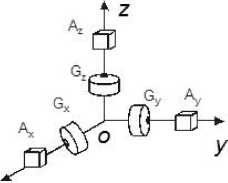
Let us consider IMU of strapdown INS [13] (Fig.1) consisting from a triad of single degree-of-freedom gyroscopes G , G , G and a triad of accelerometers A , A , A that are mounted to a vehicle with body frame oxyz with orthogonal sensitivity axes, as shown on Fig. 2.

Taking into consideration the errors of instruments (biases, scale-factor errors), mounting misalignments of the gyroscopes and accelerometers, which cause crosscoupling terms, and in-run random bias errors, the gyro’s output signals may be expressed as shown below:

\U- 1		Г B. 1		o x		" wox "
U-	=	B rny	+ K ■	. y	+	w m y	.          (1)
U |_  .Z J		B .z		_® z _		_ w .z _

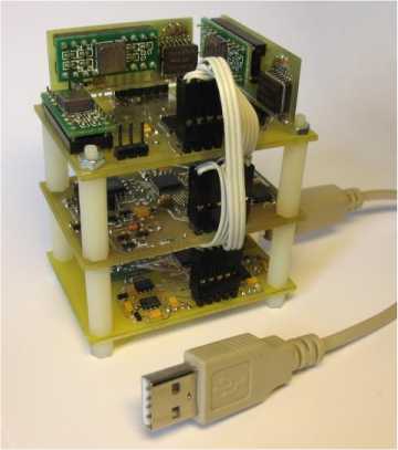
Fig.1. Inertial measurement unit with USB-port

Accelerometer’s output signals also may be expressed as shown below:

Uax Bax ax wax Uay = Bay + Ka • ay + way ,         (2) . Uaz_ _ Baz _ _ az _ _ Waz_ where U^a)x , Um(a)y , U«(a)z - is a set of output signals of gyroscopes (accelerometers), tox ,toy ,toz - are the applied angular rates acting about the principle axes of the vehicle, a ,a ,a - are the accelerations acting along these same axes, Bto(a)x , B«(a)y , B«(a)z " is a set of the residual fixed biases of gyroscopes (accelerometers), wm

X

Fig.2. Inertial measurement unit

Let us assume that calibration of IMU has being done before and all above mentioned parameters like as residual fixed biases, scale-factor errors and mounting misalignments angles of gyroscopes and accelerometers are measured and reserved in internal INS computer’s memory.

U. = b +(S + E )Q x+S a xz Qy - S Axy Q-.+ w ;

UQy = B„y+(Stoy+Etoy) Qy - Stoy Ayz Qx+Stoy A„ Q+w^;

UQ = Btoz + (Stoz + Etoz )Q + Stoz AzyQx - Stoz A . Qy + Wqz ,

K

ω

Stox^{+ E}tox - Stoy^Ayz StozA zy

^Stox^Axz Stoy⁺Etox - Stoz^Azy

^-Stox^Axy Stoy A yx

Stoz⁺Etox

K

a

- Say^Ayz Saz A zy

Sax A_   -Sm A„ ax xz          ax xy

Say + Eax   Say A yx

^-Saz^Azy   ^Saz^{+ E}ax

U =B +(5 ^E )я +£ A g -S A g +w ;

gx      ax      ax     ax gx     ax xzgy     ax xygz     gx ;

U =B +(5 +E -^ A g +5 A g +w ;

gy      ay      ay     ay gy     ay yzgx     ay yxgz     gy ;

^Ugz = Baz^{+ (S}az^{+ E}az ) ^gz^{+ S}az^Azy^gx - ^Saz^Azxgy⁺wgz ,

Fig. 3 and Fig. 4 shows examples of output signals of gyroscopes and accelerometers of IMU with USB-port [13] on stationary base.

Gyro Output signals

i^*WN^^

0             500           1000           1500           2000           2500           3000           3500           4000

points

0             500           1000           1500           2000           2500           3000           3500           4000

points

0             500           1000           1500           2000           2500           3000           3500           4000

points

Fig.3. Output signals of gyroscopes ADXRS22295 (Gx and Gy) and ADXRS300 (Gz) on stationary base.

points

points

points

Fig.4. Output signals of accelerometers ADXL202 (Ax, Ay and Az) on stationary base.

Let's divide every expression of output signal of accelerometer on corresponding scale factor and vector's module g (g = g2 + g2 + g2 ) and every expression of output gyro signal on corresponding scale factor and vector's module Q (q = ^Q^+Q^+Q2). Above two sets equations (3) and (4) are similar by form and therefore it will be enough to consider accelerometer’s output signals (4) only after normalization:

U, В ( E ^ 9     g     9   w_

--gx_ =      + 1 + -  gx + Д ^-  л  gz + __g_ ;

y ax g     ax g \     ax J g        g        g     ax g

^Ug=^B₊f₁₊^E1gy.__Д  g__Д  gz.₊w

Say • g   Say • g I   Say J g     yz g    yxg   Say " g

U   В ( E ^ 9   9   gw

--gL_ = —a— + 1 + _sz gz. + д gx _д Ay + —gL_. Saz • g   Saz • g I   Saz) g     zy g       g   Saz' g

Let us to input new denotations of dimensionless output signals and values of right parts as follows:

Ugj          gj        Baj        Eaj        wgj

’  SajS" gj g      S.g ■’   S.”S.g ■

U »      »       B-j      E-j u = ——;Q, = —L; b = ——;e,,• = —-;n = ——. » S-Q j Q  » S-Q - S-;^

Here j = x, y, z.

Using above denotations (5) the normalized accelerometer’s output signals can be described as и  = b + (l + e    +A g -A g -vn;

gx     gx         ax  gx     xzgy     xygzgx и =Ь + (l + e    -A g +A g in;

gy     gy          ay  gy     yzgx     yxgz     gy;

и = b + (l + e    +A g -A g in.

gz     gz          az  gz     zygx     zxgy     gz .

After removal of brackets we will have и     +6 +77 +e g +A g -A g :

gx   gx gx    gx axgx     xzgy     xygz ;

и —g -vb +n +e g -A g +A g ;

gy   gy gy    gy aygy     yzgx     yxgz ;

и -g +/7 +72 +e g +A g -A g . gz   gz    gz gz    azgz     zygx     zxgy .

According to scalar method of calibration [10, 11] let us sum of squared of normalized accelerometer’s output signals as following below

222 ugx⁺ugy⁺ugz =

[gx⁺ (bgx⁺ngx⁺eaxgx^{+ Д}xzgy^{- Д}xygz )] ⁺

[gy^{+ (Ь}8,-⁺ngy⁺eaygy — ^Дyzgx^{+ Д}yxgz )]^{2 +}

[gz⁺ (^bgz⁺ngz⁺eazgz^{+ Д}zygx — ^Дzxgy )]² •

It is necessary to calculate the scalar value of measuring vector and compare it to the known scalar value of measurable vector. For that let us remove of brackets in right side:

u 2 + u 2 + u 2 = g 2 + gx     gy     gz gx

(b +n +e g +A g -А ё1 + gx gx    gx    axgx     xzgy     xygz

⁺(^bgx⁺”gx⁺eaxgx^{+ Д}xzgy^{_ Д}xygz )^{2 +}g^ ⁺

²gy^(bgy⁺”gy⁺eaygy ^_Дyzgx^+Дyxgz⁾⁺        (6)

(^bgy⁺ngy⁺eaygy^{_ Д}yzgx^{+ Д}yxgz )^{2 +}gz⁺

²gz (^bgz⁺ngz⁺eazgz^{+ д}zygx^{_ Д}zxgy ) ⁺

(b -vn +e g +A g -A g 1 .

gz     gz     azgz     zygx     zxgy .

As far as g2 + g2 + g2 = 1, and also ignoring values of the second order to the trifle like (...)2, for the triad of accelerometers will get

2 ⁽ugx⁺ug- ⁺ugz^{_ 1)}=

(b -vn +(b -vn +(b -vn Xg + gx    gx gx     gy    gy gy     gz    gz gz

^+eax^glx⁺eaygy⁺eazgz^{+ 5}a 18x8y^{+ 5}a2gxgz^{+ 5}a3gygz ,

Where

J,=A -A ,A₉=A -A ,A,=A -A . a1       xz yz , a2       zy       xy , a3        yx       zx .

For the triad of gyros (»2 +Q2 +Q2 = 1) analogically will get

- ( u Qx^{+ U г}_Пy^{+ U} k- 1) =

⁽bOx⁺nOx^)Qx^{+ (Ь}Оy⁺nq_v^)Qy^{+ (}bQ + nq^)Qz⁺

+e„x Ox + e_my Q y + eJQ Z + 3_Ю10 x Qy + 3_{m 2}O x O z + 3_тзО _yQz •

Here

3, = A -A ,3 . = A -A ,3 л = A -A o1       xz      yz, оZ       zy      xy,  cd3       yx      zx

Hence, the difference between the scalar value of the normalized measurable vector and his actual value that is equal to one, proportional to the errors of the inertial instrument cluster. Coefficients in this dependence are the normalized values of measurable acceleration g ,g ,g for accelerometers and angular rate

Q_x, Q , Q_zfor gyros, their exponential orders and compositions.

On the base of equations (7) and (8) let us build the algorithm of scalar method of quality monitoring for triad of accelerometers and gyros. For sampling time t it is possible to establish following below predicates:

F0g⁽tk ) = ^Л0g |-(ugx⁺ugy⁺ugz - ^{1) - A}0g j = |₀,

FOO⁽tk ) = ^ЛOQ | 2 ⁽uQx⁺uOy⁺uQz  ¹⁾- A)O

Here in right part a value ‘1’ is mean an operable state of a triad of accelerometers or gyroscopes, a value ‘0’ – a his failure,  Ag  —

“ ( u 2 + u 2 + u 2 - 1)  • gx     gy     gz

(ugx+ug+ug-1) win

a border value of function

If the value of function not more than a value 2Ag , therefore a triad of accelerometers has being in operable state. If not, therefore there is a failure. The same rule is valid for quality monitoring of gyros.

When the task of the quality monitoring is solved it is necessary to find a place and clear the reason of failure.

For that 18 unknown parameters should be found from equations (7) and (8). These 18 parameters are distorted of the inertial instrument cluster output signals. Six of them are differences of mounting misalignments angles of the devices.

According to scalar calibration of the inertial measurement unit we should in the gravity field to turn around certain direction at fixed angles and in every position get the normalized output signals. To solve the equations (7) and (8) it requires at least nine of the inertial instrument cluster position, so number of tests should be more or equal of nine. The fact is that in each one position of the inertial instrument cluster its output signals simultaneously have been measuring either gyroscopes or accelerometers, so the minimum number of positions in the two times less than the total number of required parame- ters.

Consider the equation (7) and (8) in matrix form for n - testing operations or measurements:

Ug = ^G• eg,  “q = Qen,            ⁽⁹⁾

where u_a, u_gis a n x 1 column vectors of the normalized inertial measurement unit output signals:

ug

2 (ugx i+ug i+ugz• i—1) - (ugx 2+ug 2+ugz 2—1)

G , Q - is a n x 9 i of the acceleration g a		atrixes of normalized projections
		ind turn rate Q	of dimension:
	gx 1	gx2	gxn
	gy 1	gy2	gn
	gz 1	gz2	gn
	gx21	gx22	gL
GT =	g21	gy22	g,.	;
	gz2	gz22	. Szl
	gx 1 gy 1	gx2gy2	gxngyn
	gx 1 gz 1	gx2gz2	gxngzn
	_ gy 1 gz 1	gy2gz2	gyngzn
	■ Q x 1	Qx 2      • • •	Q " xn
	Oy 1	Qy 2      • •'	Q yn
	Q.• 1	Q,. z	Q zn
	Q 21	Q22	Q2 xn
Q' =	O 21	O 2 z   -	Q2n	;
	qz 1	Qzz	2 zn
	Q x 1Q y 1	Qx 2 Qy 2	Q Q xn   yn
	Qx 1Q z 1	Qx 2 Qz2  -	Qxn Qzn
	Oy 1Qz1	Qy 2 Qz 2	Oyn Qzn _

gxn     gyn     gzn

1( uOx 1 + u Qy 1 + u Qz 1 -1) u«= 2 ( u Ox 2 + u Qy 2 + u Qz 2 - i) 2 ( u Qx n + uQyn + u Qzn • -1) eg, ef- - is a 9 x 1 column vectors of unknown parameters

Solving the matrix equation (9) by least-squares method, we obtain:

eg =(GTG rGTUg^,

, en =(^T^)- nTufi

where eˆ , eˆ - is an estimating values of the unknown parameters of inertial measurement unit.

Thanks to the least squares method the results are smoothing, and as long as average of distribution is equal to zero

M {nx }= M {n }= M {nz } = 0, then estimated values eˆ , eˆ will not have a random noise:

.

According to introduced relationships (5) we can calculate estimations of B„(a)x , B„(a)y,, B„(a)_z and Ea(a)x , ^E_m(a)y , ^E_m(a)z as follows:

ˆ aj

/X/X

ˆˆ gj  ajg;      aj      aj aj ;

ˆˆˆ toj      Пj coj   ;      toj      coj coj

When estimated values (12) are calculated, it is possible to use following set of predicates, which are expressed the algorithm of diagnostics of gyroscopes triad on stationary base:

Fln ( tk ) = ^ЛC {| ^Bax^{— B}ax\^-An} =   ;

F2n⁽tk ) = ^ЛП {|^Bay - Bay | ^-An} =   ;

M tk )=Л_П{| Bi ax - Bax | ^-Ad}^

^F4n ⁽tk ) = ^ЛП {|^Eax^{- E}ax | ^{- A}4n } = ^q^;

F5n( tk )=Л_П{| E?ay - Eay\ -A_5n}={1;

^F6n⁽tk ) = ^ЛП {|^Eaz^{— E}az | ^—Абд } = ^Q ^;

^F7tl⁽tk ^{)= Л}Cl {| Bal ^—Bal | ^- Лй} = ^q^;

^F8n⁽tk ) = ^ЛП {|Ba2 ^—Baz| ^-Лп} =   ;

F9n( tk ) = Л_Й{| Bia 3 — Ba з| - ^9^}=^!.

Here A, Aci, Ad — border values of gyro biases, Ad, Ad, Ad — border values of gyro scale factor errors, Ad, Ad, Ad — border values of gyro mounting misalignments. If the difference between calculated values eˆ will not more than a values ±A , therefore a triad of gyroscopes has being in operable state. If not, therefore there is a failure. The number of eˆ , which are excited out of value ±A , indicate not only what gyro is failure, but also indicate a reason of failure: excessing of real biases, scale factor errors or mounting misalignments to their nominal values.

The scheme of scalar method of fault diagnosis systems of IMU is depicted in the Fig. 5. Here numbers 1, 2, 3 is shown the gyro’s failures via biases discrepancy, numbers 4,5,6 - gyro’s failures via scale factor errors discrepancy and numbers 7,8,9 - gyro’s failures via mounting misalignments discrepancy.

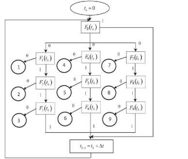
Fig.5. Scheme of scalar method of fault diagnosis systems of gyro’s triad IMU

• III.    The Scalar Diagnostics on the Moving Base

Let us consider scalar diagnostics on the moving base. Using initial equations (1) and (2) we can receive following relations for gyro cluster

^Umx = ^Bmx + ^(Smx + ^Emx ) ®x + ^S_mx^Axz®y - ^S_mx^Axy®z + wmx ;

^Umy = ^Bmy + (^Smy + ^Emy ) ®y - ^Smy^A.z® + ^Smy^Ayx^z + w^y ;

Urnz = Bmz + (Smz + Emz ) ®z + SmzAzy®x - SmzAzx^y + w^z , and for accelerometer’s cluster

^Uax = ^Bax^{+ (S}ax^{+ E}ax ) ax^{+ S}ax^Axzay - ^Sax^Axyaz⁺wax ;

U = В + (S +E -S A a +S A a +w ;

ay      ay       ay      ay y     ay yz x     ay yx z      ay ;

^Uaz = Baz^{+ (S}az^{+ E}az ) az^{+ S}az^Azyax - ^Saz^Azxay⁺waz •

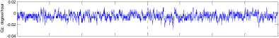
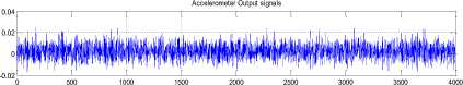
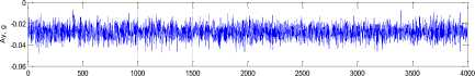
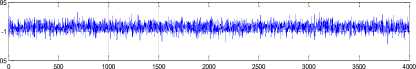
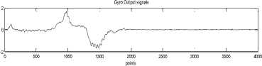
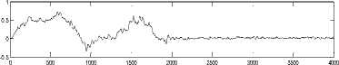
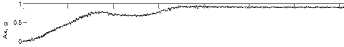
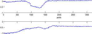
Fig. 6 and Fig. 7 shows examples of output signals of gyroscopes and accelerometers of IMU with USB-port [13] on the moving base (takeoff with sharp turn).

points

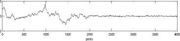
Fig.6. Output signals of gyroscopes ADXRS22295 (Gx and Gy) and ADXRS300 (Gz) on the moving base.

Accelerometer Output signals

-0.5

500           1000           1500          2000          2500          3000

points

3500          4000

3500          4000

-1.5

0            500           1000           1500          2000          2500          3000           3500          4000

points

Fig.7. Output signals of accelerometers ADXL202 (Ax, Ay and Az) on the moving base.

According to scalar diagnostics method let's divide every expression of output signal of accelerometer on corresponding scale factor and vector's module a = 4a2 +a2 + a=2 and every expression of output gyro signal on corresponding scale factor and vector's module to = X / ®x + ®2 + ®z • xyz

New denotations of dimensionless output signals and values of right parts will be as follows:

Uaj	a =-; baj = a	Baj
uj= Sja1  aj		Saja;
E e . = —-;n . = ajaj Saj m, m = — ; b™j m	n aj	Uj.
	;u S4a   " =Bmj^; e	Smj® E®l.	(16)
	Smj®’m	Smj’
nml
nmj    c     • Smj®

Here j = x, y, z.

On the stationary base we should to use magnitude of gravity vector g and Earth's rate Q . But how we can get current values of a.,a,,,a, and m ,ю ,m on the xyz     x y z moving base for calculations of a = Ja2 + a2 + a2 and to = x Z®2 + ®2 + юЮ ?

xyz

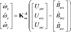
Solving equations (1) and (2), we can receive estimated values <y_v, <y,,, <y,: xyz

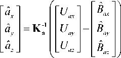
Also estimated value of the

1                           /X /X /X accelerations a ,a ,a xyz

could be calculated as

Now we can receive a = . № + a2 + a2   and xyz to = . Ito + to + to . xyz

As far as on the moving base for the triad of gyros юг²+ ®2 + Ю²= 1 we will have following equation:

12       22

2 \ mx    my

(bmx + nmx )mx + (bmy + nmy )юу + (bmz + nmz )Юх

+emxmx + emymy + emzmz +

8rni^mx^my⁺8_ffl2^mx^mz⁺8_ffl3^my^mz •

For the triad of accelerometers a2 + a2 + a2 = 1 will xyz get us similar equation:

— (u²+ u²+ u²-1) = ax     ay     az

⁽bax⁺nax )ax^{+ (}bay⁺nay )ay^{+ (b}az⁺naz )az⁺    ₍2₀₎

⁺eaxaX⁺eayay⁺eazaZ⁺

⁵a 1 axay^{+ 5}a2axaz^{+ 5}a3ayaz •

u

12        2        2 2 ( uax 1 + uay 1 + uaz 1	-1)
12        2        2 — 1 I n + U n + U n ax2      ay2      az2	-1)
1 222 axn     ayn     azn	-1)

Hence, the difference between the scalar value of the normalized measurable vector and his actual value that is equal to one, proportional to the errors of the inertial instrument cluster. Coefficients in this dependence are the normalized values of measurable acceleration av,a .a for accelerometers and angular rate to,ю,,to xyz                   xyz for gyros, their exponential orders and compositions.

Analogically to algorithm of scalar monitoring on the stationary base, from equations (19) and (20) we can build the algorithm of scalar method of quality monitoring for triad of accelerometers and gyros for moving base. For sampling time t it is possible to establish following below predicates:

F0a (tk ) = Л0a |“(uax + uay + ^z - —) - A0a ^ = ^Q ,^^

u

" 1Л, 2 2(utox 1	+utoy 1	+utoz 1	-1)
1Г 2 2 ( utox 2	+ uray 2	+ utoz г	-1)
....... 1/  2 — \u 2 \ toxn	2 toyn	2 tozn	• -1

A , to - is a n x 9 matrixes of normalized projections of the acceleration a and turn rate to of dimension:

K-At, ) = Л0| — (u2 + u2 + u2 -1) - A 1 = 1 .

Oto \ kJ      0 2 ' tox     toy     toz     /     O®Q

Here in right part a value ‘1’ is mean an operable state of a triad of accelerometers

or gyroscopes, a value ‘0’ – a his failure, Aa -

1_{2      2      2}

— \ ll + и + и ax     ay     az

^-1)  •

(^uax⁺"to ⁺"to ^{- 1}) ^will

a border value of function

If the value  of  function not more than a value 2Ag , therefore a triad of accelerometers has being in operable state. If not, therefore there is a failure. The same rule is valid for quality monitoring of gyros.

When the task of the quality monitoring is solved it is necessary to find a place and clear the reason of failure.

For that 18 unknown parameters should be found from equations (19) and (20). These 18 parameters are distorted of the inertial instrument cluster output signals. Six of them are differences of mounting misalignments angles of the devices.

Consider the equation (19) and (20) in matrix-block form:

			ax 1	ax2	•     axn
			ay1	ay2	•     ayn
			az1	az2	•      azn
			ax21	2 ax22	2 xn
AT	=		ay21 az21	ay22 az22	■     ayn •      azn
			ax1ay1	ax2ay2	•   axnayn
			ax1az1	ax2az2	•   axnazn
			L ay 1 az 1	ay2az2	•   aynazn _
		г	tox 1	tox 2       •	•      toxn   "
		toy 1		toy 2      •	•      toyn
		toz 1		toz 2       •	•      tozn
		— 2 tox1		tox2       •	.      to2 xn
ωT	=	toy1 toz21		toy2      • — 2 toz2       •	— 2 •      toyn .      tozn
		tox 1toy 1		toto x2  y2	■   toxntoyn
		tox 1toz 1		tox 2toz 2    •	•   toxntozn
		L	toy 1toz 1	toy 2toz 2    •	•   toyntozn _

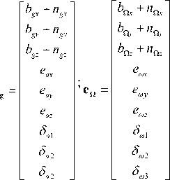
e_a, e_to - is a 9 x 1 column vectors of unknown parameters

u = A • ea, aa

^, ωω

where u_a,u_fiis a nx1 column vectors of the normalized inertial measurement unit output signals:

	bax+nax		b„x+ n„x
	bay+nay		b„y+ntoy
	baz+naz		b«,-.+ n™z
	eax		etox
ea =	eay	; e«, =	еЮу
	eaz		e„z
	5a 1		5.
	5a 2		5m 2
	5a 2		5„з

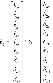
Solving the matrix equation (23) by least-squares method, we obtain:

where eˆ ,eˆ - is an estimating values of the unknown parameters of inertial measurement unit.

Thanks to the least squares method the results are smoothing, and as long as average of distribution is equal to zero

^F5a (t_k )=^Лa {| E?a, — ^Ea,| < ^5 a } = ^ F6a (tk ) = A a {| Eiaz — Eaz\< ^6 a }= ^ F7a (tk )=A a {| Bia 1 — 5a J < X, a } = {^; F8a (tk )=A a {| 5a 2 — Ba 2| < X8 a } = ^ F9a (tk ) = A a {| 5a 3 — Ba з| < Л9 a } = |1-

M {nx } = M {n, } = M {n}= 0, then estimated values eˆ , eˆ  will not have a random noise:

_a, _ω

According to introduced relationships (16) we can calculate estimations of B,(a)x , B(a), , B,(a)_z and ^E™(a)x , EX(a), , ^E_m(a)z on moving base as follows:

В = b Sa; E = e S ;

aj      gj aj          aj      aj aj

ˆ toj       Qj  toj   ;      ^j      ^j  toj.

And algorithm of scalar method of diagnostics of accelerometers triad will correspond to predicates

F1a (tk )=A a {| Bia — Bax\< X a }= ^ ^F2a (tk )=A a {| Biay — Bay | < ^ a }= ^ Fa (tk )=Л _a {| Bi_az - Baz\< X a j^ F4a (tk )=A a {| Eax — Eax| < ^4 a }= ^

Here Xa, Xa, Xa — border values of accelerometers biases, Xa, Xa, Xa — border values of accelerometers scale factor errors, X_a, X_a, Xa — border values of accelerometers mounting misalignments. If the difference between calculated values e will not more than a values ±X , therefore a triad of gyroscopes has being in operable state. If not, therefore there is a failure. The number of eˆ , which are excited out of value ±X, indicate not only what gyro is failure, but also indicate a reason of failure: excessing of real biases, scale factor errors or mounting misalignments to their nominal values.

• IV.    Conclusions

In this paper we have proposed a new method of fault diagnosis of Strapdown Inertial Navigation Systems. The scalar calibration method is a base of the scalar method of quality monitoring and diagnostics. Algorithms of fault diagnosis systems are developed in accordance with scalar calibration method. In result of quality monitoring algorithm verification is implemented the working capacity monitoring of IMU. A failure element determination is based in diagnostics algorithm verification and after that the reason of such failure is cleared.

The process of verifications consists of comparison of the calculated estimations of biases, scale factor errors and misalignments angles of sensors to their data sheet certificate, which kept in internal memory of computer. In result of such comparison the conclusion for working capacity of each one IMU sensor can be made and also the failure sensor can be determined.

Acknowledgements

I am thankful to Mr. Bob Sulouff, Vice-President of Analog Devices Inc. ® and his team for great support and samples of ADI gyroscopes and accelerometers.

I am very grateful to Dr. Oleg Stepanov, Professor of St. Petersburg ITMO University for time in Ladoga and kind comments.

Also I am thankful to my parents and my family who have always believed me.