Service-based analysis and processing of meteorological data for environmental monitoring of natural territories

The effective solution of current scientific and technological challenges depends on detailed and reliable initial information. The specifics of such information depend on the domain of human activity and the subject of research. Relevant energy-related issues involve the development and operation of energy complexes and systems, especially with the growing integration of Renewable Energy Sources (RES). The analysis of operation modes, economic aspects, environmental monitoring, and other impacts of RES requires comprehensive meteorological data for the considered territory.

Understanding the current state of natural territories and forecasting their potential development direction often requires high-quality meteorological data [1]. The extraction, analysis, and interpretation of large amounts of both current and retrospective meteorological data, together with information on climate change, are extremely useful for effective natural resource management and for reducing the risks associated with extreme weather conditions in various regions and sectors [2–4]. In particular, solving problems related to the sustainable development and operation of natural and technical systems depends on access to detailed climate data, including important parameters such as wind speed and direction, solar activity, pressure, temperature, humidity, air density, cloudiness, and other indicators. Such data are also essential for environmental monitoring problems [5], where models of a typical, optimistic, or pessimistic meteorological year play a key role. These models are designed using reliable retrospective data, which requires correction and elimination of various inaccuracies. Detection and correction of missing [6, 7] and anomalous [8] values in meteorological time series, and correcting them, is crucial to ensure the accuracy of climate forecasts.

This is particularly important for archived meteorological records, which often include distorted values due to technical malfunctions, measurement errors, or extreme weather events. The reliability of data for a specific location can be improved by using information from nearby weather stations. However, accessing retrospective meteorological data can be time-consuming, making it essential to use flexible and efficient tools for data extraction and processing from open sources. Such data may include multi-year time series represented as a multidimensional matrix, where each column represents a parameter, and each row represents a numerical value or textual description. Land-based hydrometeorological stations use the FM 12 SYNOP international code [9], which has the predefined structure and sequence for storing meteorological data. Extracting and processing this information (correcting inaccuracies, filtering out outliers, and filling in missing data) are essential steps in reconstructing the climatic conditions of the region under study. The reliability and accuracy of such data are critical because many problems rely on environmental and climatic information as a starting point that directly influences the final outcome. For example, the problem of optimizing the equipment configuration of a solar power plant depends on the results of modeling the generation of photovoltaic systems, where the key parameter is the total solar radiation incident on the given territory. As an illustrative example, consider the actinometric data for the settlement of Bur (Katangsky District, Irkutsk Region). According to publicly available sources such as NASA POWER and PVGIS, the annual total solar radiation on a horizontal surface ranges from 1250 to 1300 kWh/m². At the same time, a detailed actinometric atlas of the Irkutsk Region, developed by the Institute of Geography of the Russian Academy of Sciences, which takes into account terrain features and other local conditions, shows that the average annual value of total solar radiation does not exceed 950 kWh/m². The Scientific and Applied Climate Reference Book of the USSR provides average values of up to 1000 kWh/m².

Thus, the discrepancy between open-access online sources and locally validated data is about 30%. Various web applications [10] and services [11–14] are widely used to implement the processes of obtaining, processing, storing, and analyzing spatially distributed data [15]. In particular, [11, 13] present services for forecasting climatic conditions and assessing their impacts on environmental management. However, an analysis of such studies shows that the issues of automating the construction of service compositions, providing flexible access to services both via a web interface and through a specialized API, supporting the WPS standard, and implementing many other aspects remain open. In this context, we have developed an application with a suite of web services for acquiring, processing, and analyzing multidimensional meteorological time series from open sources. The application implements the Web Processing Service (WPS) standard [16]. Unlike other web services, WPS is specifically designed to handle spatially distributed geospatial data. It supports real-time execution of complex computations and allows monitoring of the processing status. The development of WPS services is justified by the need for their integration with geographic information systems (e.g., the geoportal of IDSCT SB RAS) that support the WPS standard.

In this context, the following aspects define the essence and novelty of the proposed approach:

• • The use of the WPS standard enables processing of spatially distributed geospatial data, supports real-time execution of complex computations, and provides mechanisms for monitoring service execution status.

• • The Framework for Development and Execution of Scientific WorkFlows (FDE-SWFs) allows for modeling application logic as workflows and executing them in a heterogeneous, distributed computing environment.

1.    Preparation of multi-year meteorological series

The study of climatic conditions and their influence on various processes and systems involves a technology that encompasses the collection, analysis, and processing of meteorological data. These data describe the temporal dynamics of various environmental parameters. The process of forming multi-year meteorological series includes the following key stages:

• • Retrieving multi-year meteorological data sets;

• • Analyzing and processing the meteorological data;

• • Forming the final dataset of environmental parameters.

The extraction of multi-year meteorological datasets is carried out through a service that retrieves climate data from an external meteorological information system. The retrieved datasets are then processed and analyzed for missing or anomalous values. Based on the cleaned dataset, along with mathematical models and supporting meteorological information, the final multi-year dataset of parameters is generated. This dataset includes actinometric, wind energy, and other indicators according to the international FM 12 SYNOP coding standard. The overall technology for compiling multi-year meteorological datasets is illustrated in fig. 1.

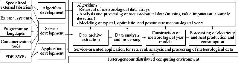
Fig. 1. Application development technology

The FM 12 SYNOP code includes the following parameters that change over time: wind speed and direction; air temperature; atmospheric pressure; humidity; cloud cover and other meteorological indicators. These variables are expressed as a function h t (t), where i denotes the parameter index and t is the time of observation. The code conventionally contains two types of information: a dataset of measured meteorological variables and a verbal description of cloudiness by cloud layer. Additional data on the vertical thickness of the ozone layer, as well as the presence of liquid water and vapor droplets in clouds, are also incorporated. These data can be obtained from open-access archives such as the World Ozone and Ultraviolet Radiation Data Centre (WOURDC) [17] and AERONET [18]. This information is critical for achieving accurate estimates of the actinometric properties of a given region. A more detailed mathematical description of the preparation of multi-year meteorological series using the FM 12 SYNOP code, along with its application in energy research, is provided in [19].

Solar radiation on a horizontal surface is influenced by several geographical and astronomical factors, including latitude, longitude, sunrise and sunset times, and time zone. Latitude and longitude determine the angle of solar incidence and the duration of daylight, which in turn affect total solar radiation. In addition, time-varying weather conditions have a significant impact. For example, extensive cloud cover can greatly reduce direct solar radiation. The composition of clouds (especially their water vapor and aerosol content) also affects the extent of scattering and absorption of solar energy. Furthermore, the albedo of both clouds and the Earth’s surface influences the levels of diffuse and reflected solar radiation. Two mathematical models are used in this study to simulate solar radiation: the Iqbal model and the Kasten-Czeplak model [20]. The Iqbal model is used at the initial stage to simulate solar radiation under clear sky conditions. Subsequently, the Kasten-Czeplak model is applied to determine the radiation attenuation coefficient, which depends on cloud cover, cloud composition, and the proportion of foul-weather clouds.

The concept of a typical meteorological year forms the basis of standard methodologies used in solving technical problems, particularly in the field of energy systems [21]. This concept has become especially prominent in international commercial software packages (e.g., PVscout, PVSOL, PVsyst), which are used for modeling solar heating systems, air conditioning processes in buildings, and renewable energy infrastructure [22]. A typical meteorological year is an artificially constructed year based on long-term meteorological records and the modeling of individual parameters. It represents the average climatic conditions of a given location but does not capture the occurrence of extreme values for specific variables across different seasons, months, or days [23].

Therefore, the identification of an extreme meteorological year is essential to address issues related to the operational performance, structural reliability, and resilience of technical systems [24]. This is particularly relevant for renewable energy facilities, where the reliable operation of photovoltaic systems is highly dependent on external climatic conditions. For example, strong wind loads can affect the structural integrity of supporting frameworks in solar power plants. Extremely low temperatures can affect the voltage output of photovoltaic modules. The presence of precipitation and high humidity during freezing events can also be critical. Consideration of the extreme values of meteorological indicators with their seasonal variation and recurrence is critical to evaluating the feasibility of potential technical solutions. This allows for informed assessments of system reliability, survivability, and techno-economic efficiency. The modeling process uses climate datasets formatted according to the FM 12 SYNOP meteorological code. These datasets are structured as matrices containing instrumental measurements (Д „ ) and qualitative assessments of annual cloud cover (B^T) for the target calculation period ( τ ):

^ m    [^ wind , f air , Vai r , ^ф % , C % , ],

Bx = [Cb Cm, ch, b%], where: Vw[nd is wind speed at 10 meters height, m/s; Tair is outdoor air temperature, °C; Vair is atmospheric pressure, mmHg; ф% is relative humidity, %; c% is total cloud cover, %; Cl, Cm, Cb are clouds of low, middle, and high tiers, respectively; b% is percentage of bad weather clouds.

Using these datasets, key parameters describing atmospheric processes in the middle and lower layers of the troposphere are derived. These parameters are then applied to calculate the total solar radiation (W/m²) for each hour of the calculation period ( t ):

I t (t) =I _b (t)+I d (t), (3) where: I _b (t) is a direct solar radiation measured in W/m²; I _d (t) is a diffuse (including reflected) solar radiation measured in W/m².

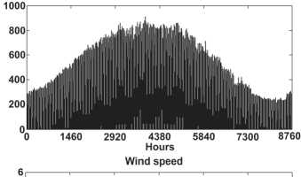
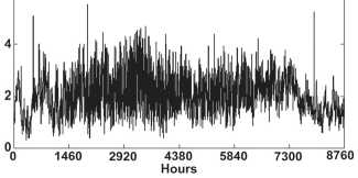
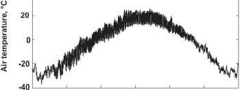
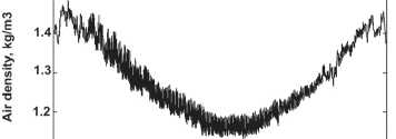
A detailed explanation of this calculation methodology, including data verification for different locations, along with assessments of its reliability and applicability for energy system planning and operation, is provided in [25]. As an illustrative example, fig. 2 presents the characteristics of a typical meteorological year constructed from long-term FM 12 SYNOP data series for a settlement located in Eastern Siberia. Extreme meteorological year characteristics are also derived from these multi-year time series. In this case, the key parameters include outdoor air temperature, wind speed, and total solar radiation. The entire available dataset is examined, with key parameters highlighted for both optimistic and pessimistic meteorological years.

2.    Application architecture

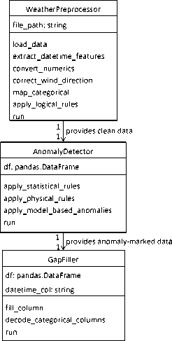
The application is implemented using FDE-SWFs [26]. This framework is a workflow management system. In the course of the application design, we developed UML diagrams that capture the system architecture, its behavioral aspects, and the interactions among components. fig. 3 a shows an activity diagram that describes the sequence of operations in the anomaly-processing and gap-filling workflow, making the control flow of the module explicit at the behavioral level. Next, a component diagram that shows the decomposition of the system into functional modules and the interfaces through which they interact is presented in fig. 3 b . Finally, fig. 3 c demonstrates a class diagram that presents the structure of the core classes implementing these functions, including their attributes, methods, and relationships.

The interaction between the architectural components is organized as follows: a user submits a request to the application through the geoportal. The application processes the request by initiating the execution of the appropriate services or service compositions. Some services access external data systems to retrieve additional information or to invoke external software systems. Upon completion, the application returns the results of the service execution to the geoportal. Users then access the computational results through the geoportal interface. The implemented services and development tools are presented in tab. 1. The following service compositions are supported within the application (where arrows “→” and “↓↓” denote sequential and parallel service execution, respectively): s1 → s2; s1 → s2 → s3; s1 → s2 → s4; s1 → s2 → (s3 ↓↓ s4); s1 → s5. A demo version of the service compositions can be found at the following URL:

c)

Total solar radiation on horizontal surface

a)

b)

d)

Fig. 2. Indicators of a typical meteorological year for a conditional location.

Air temperature

40 -------------- T--------------T--------------T-----------

0     1460    2920    4380    5840    7300   8760

Hours

Air density

1.5

0     1460    2920    4380    5840    7300   8760

Hours

(a) total solar radiation, (b) air temperature, (c) wind speed, (d) air density

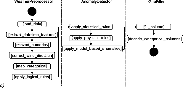
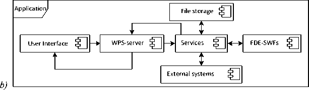
Fig. 3. UML diagrams. (a) activity diagram, (b) component diagram, (c) class diagram

Tab. 1. Services

Service Description	Development Tools
Retrieval of meteorological data arrays from a weather site rp5.ru [27], filling in missing values, and mitigating anomalies ( s 1)	Python libraries: BS4, Requests, Pandas, and datetime, along with gzip and json modules. A regression model (DecisionTreeRegressor) is used for gap filling and anomaly smoothing.
Design of meteorological year models ( s 2)	Python libraries: NumPy, SciPy, and cmath.
Assessment of electricity generation by a solar power plant ( s 3)	Python libraries: GSEE and Pandas. Global Solar Energy Estimator [28].
Assessment of electricity generation by a wind turbine ( s 4)	Python libraries: Requests, Pandas, and datetime. Wind power generation simulation system [28].
Simulation of consistent climate time series ( s 5)	C++ libraries: Intel oneAPI Math Kernel Library and OpenMP; Python libraries: urllib and os.

3.    Processing and analyzing anomalies and missing values

A methodology for analyzing and processing meteorological time series data is proposed, comprising the following main stages:

• • Detection of missing data values and filling them in:

a.Conversion of categorical data into numerical format;

b.Training of a model to predict missing values in the time series;

c.Analysis of the time series to detect missing values;

d.Filling in missing data using the trained model.

• • Detection and mitigation of anomalies in time series data:

a.Normalization of data;

b.Analysis of the time series to detect individual anomalies;

c.Mitigation of individual anomalies;

d.Detection of contextual anomalies in the time series;

e.Mitigation of contextual anomalies.

A meteorological time series is a sequence of observations of specific parameters recorded at regular intervals. Such data are critical for identifying patterns, analyzing trends, and predicting future values. The detection of missing data values and filling them in are essential components of time series analysis. In this research, a regression model based on a decision tree [29] is used. This model is effective for capturing nonlinear dependencies among features, accounting for temporal and contextual characteristics of the data, and offering high interpretability. Since decision trees do not natively support categorical variables [30], these must first be converted into numerical form.

Temporal features such as year, month, day, and hour are used as independent variables in constructing the decision tree. Temporal factors, such as seasonal and diurnal variations, often significantly affect meteorological data. Incorporating these features allows the model to capture time-specific patterns, enhancing its sensitivity to temporal variations. The trained model is then applied to predict and fill in missing values in the time series. These predicted values are used to replace missing entries in the corresponding columns, preserving the completeness and structural integrity of the dataset. The categorical features that have been converted to numerical form are then restored to their original textual representation.

The anomaly detection process involves identifying both point-wise and contextual anomalies and correcting them as necessary. A critical preprocessing step for data recorded on varying measurement scales is normalization, which ensures that all data are standardized to a common scale [31]. In this study, all features are standardized using Z-score normalization prior to anomaly detection, ensuring consistent scaling and eliminating bias caused by differing units of measurement.

For detection of individual anomalies, the K-Nearest Neighbors (KNN) algorithm is employed [32], chosen for its interpretability, flexible configuration (such as the number of neighbors and distance metric), and adaptability to the data structure. The method assumes anomalies are points with significantly lower local density compared to the rest of the data. Specifically, Euclidean distance is used as the metric in the multi-dimensional feature space. The number of neighbors is empirically set to 6. This parameter influences the sensitivity of the model: too few neighbors may lead to excessive detection of anomalies, while too many can reduce the ability to identify real outliers.

For each data point, the distances to its k nearest neighbors are computed, and a Z-score of these distances is calculated [33]. If the Z-score exceeds a predefined threshold (empirically set at 3 in this study), the point is classified as anomalous. Unlike individual anomalies, contextual (group) anomalies occur within specific temporal intervals, such as days, months, or quarters [34]. To detect these, mean values and standard deviations of relevant meteorological parameters are computed for each time segment. Data points that significantly deviate from these temporal norms are identified as contextual anomalies. Detected anomalies – both individual and contextual – are corrected using predictions from the decision tree regression model described previously. This approach allows for the consideration of seasonal fluctuations and other temporal features inherent in the data.

The algorithms for filling in missing values and detecting individual and contextual anomaly are implemented in Python. Python provides a large spectrum of open-source libraries that greatly facilitate the development of machine learning and data processing workflows. The algorithms for filling in missing values use the Pandas, Scikit-Learn, and FuzzyWuzzy libraries [35].

Initially, the time series is loaded from an Excel file using Pandas. Temporal features (year, month, day, hour) are extracted from the timestamp column and used to train the model. Categorical data, such as cloud cover, cloud base height, wind direction, and other parameters, are converted into numerical form using predefined dictionaries covering all possible categories. To train the model for missing value imputation, a subset of the time series containing complete observations is selected. Temporal features such as year, month, day, and hour are extracted from the timestamp column and used as input variables. In addition to these, other available meteorological parameters are included to enhance predictive accuracy. Since decision trees do not natively support categorical variables, categorical data (e.g., cloud cover, wind direction) are first converted into numerical form using predefined dictionaries. For each target variable with missing entries, an individual DecisionTreeRegressor from Scikit-Learn is trained on the complete subset of data. This supervised learning approach allows the model to learn complex, potentially nonlinear dependencies and capture temporal patterns in the data. After training, the model is applied to predict and fill in missing values in the corresponding columns. Once imputation is complete, the previously transformed categorical features are restored to their original textual representation.

In this study, wind direction values were normalized to a simplified set of categories used for modeling, consisting of eight principal compass directions (N, NE, E, SE, S, SW, W, NW), along with "Calm, no wind." and "Variable direction." as additional states. The archived dataset, however, included more granular classifications – up to sixteen compass directions. To align these values with the target classification system, the FuzzyWuzzy library was employed to match each recorded value to its nearest valid counterpart based on string similarity. This process enabled automated mapping of non-standard or overly specific entries (e.g., "South-southeast") to the appropriate generalized categories (e.g., "Southeast"), ensuring consistency and compatibility with subsequent modeling procedures.

Anomaly detection and correction algorithms are also implemented using Scikit-Learn and Pandas. Normalization is performed using Scikit-Learn’s StandardScaler, which standardizes all features to a uniform scale, ensuring compatibility with machine learning algorithms. The nearest neighbors method for detecting individual anomalies is implemented via the KNeighborsClassifier and KNeighborsRegressor tools from Scikit-Learn. The anomaly threshold is derived from the Z-score computed over distances to nearest neighbors; this score indicates the extent of deviation from the mean. Points exceeding the threshold are classified as anomalies.

For group anomaly detection, monthly means and standard deviations of meteorological parameters are calculated using Pandas. The deviation of each observation from the monthly norm is then assessed, and significant deviations are marked as contextual anomalies. These anomalies are then corrected using the same decision tree regression model (DecisionTreeRegressor from Scikit-Learn).

Despite the use of standard libraries, the author’s contribution lies in the adaptation of meteorological time series to these libraries, as well as in the automation for all data processing stages.

4.    Example of the data analysis and processing

The results of the data analysis and processing are demonstrated using a model example. As a real time series, one of the datasets collected from a weather station located at the Baikal Natural Territory was selected. Based on this dataset, a noisy time series, denoted as ts₁ was generated by introducing missing values and anomalies in the following parameters: air temperature, atmospheric pressure, wind speed, and relative humidity. A processed time series, denoted as ts₂ , was then obtained by applying algorithms for detecting and filling missing values, as well as for identifying and correcting both individual and contextual anomalies in the data.

The Root Mean Square Deviation (RMSD) of the noisy and processed (i.e., after detecting and filling missing values) time series, relative to the retrospective time series, for the parameters mentioned above is presented in tab. 2. The RMSD of the noisy and processed (i.e., after detection and correction of anomalies) time series, relative to the retrospective time series, for the same parameters is presented in tab. 3.

Tab. 2. Results of Missing Value Detection and Imputation

Time Series	Air Temperature	Atmospheric Pressure	Wind Speed	Relative Humidity
ts1	4.5958	4.5644	1.4706	16.1919
tS 2	4.5578	4.5592	1.4629	16.1883

Tab. 3. Results of Anomaly Detection and Correction

Time Series	Air Temperature	Atmospheric Pressure	Wind Speed	Relative Humidity
ts1	8.0610	59.5603	5.1360	11.5824
tS 2	4.4575	4.0105	1.5493	9.4202

5. Aspects of the application implementation

Currently, there are no widely available tools that offer the necessary functionality for the automatic acquisition and processing of meteorological data archives. To address this issue, the service s 1 was developed. Based on user-provided information about a settlement or geographic coordinates, along with the desired calculation period, the service generates an archive of meteorological data. It also supports generating multiple archives for a set of locations. The resulting archives are provided to the user in RAR format. The system implements procedures for retrieving data, removing irrelevant information, and filling in missing data in Excel files. The implementation makes use of several Python libraries, including Requests, BeautifulSoup (BS4), Haversine, openpyxl, gzip, and datetime.

The service s2 designs models of typical, optimistic, and pessimistic meteorological years. The modeling algorithms are based on a modified version of the Iqbal–Kasten/Czeplak model. Originally, these algorithms were developed in the MATLAB programming environment. The main limitations of the initial implementation included a user-unfriendly format for displaying the calculation results, long execution times, and a lack of integration with meteorological data arrays for specific locations. The service s2 successfully addresses these issues. The typical meteorological year model is constructed based on archives generated by the service s1. The optimistic and pessimistic year models are derived from the best-case and worst-case average monthly total solar radiation values of the typical year, respectively. These models are implemented using the NumPy and SciPy libraries in Python.

The service s 3 is implemented using the Global Solar Energy Estimator package. Based on meteorological year data, geographic latitude and longitude, maximum electric power, and the tilt angle of a solar panel, the service calculates energy generation and outputs the results in CSV format.

The service s 4 implements queries through an external system for modeling electric power generation. Its input parameters include the calculation period, geographic coordinates of the wind turbine location, and its technical characteristics (maximum electric power, hub height, and model). Future plans include modifying this service to incorporate meteorological year models produced by the service s 2.

The service s 5 generates synthetic time series of meteorological data for a given geographic location over a specified time interval. Input parameters include the number of years, the number of measurement periods per day, the number of days in the interval, and a weather data array provided in text file format. The service is based on the use of stochastic weather generators [36].

Currently, meteorological time series can be stored in the following file formats: Excel, CSV, and TXT. In the future, it is planned to use the columnar database ClickHouse for storing the obtained time series, in order to facilitate their storage, processing, and analysis.

6.    Example of usage

A general scheme for the application of the proposed technology is illustrated in the context of constructing models of typical, optimistic, and pessimistic meteorological years, which are widely used in further scientific and applied studies. As a representative example, consider an autonomous energy system located hypothetically in Eastern Siberia, which includes a solar power plant, an energy storage system, diesel generator units, and auxiliary power equipment.

For each hour of a typical meteorological year, end-to-end simulation of the operating modes of the energy system is carried out. The primary goal is to meet the consumer's load demand using renewable energy sources and battery storage. If this condition is not satisfied, a backup source (a diesel power plant) is engaged.

Fig. 4 shows the structure of the autonomous energy system incorporating conventional power units, renewable energy sources, and an energy storage system. The maximum consumer load is 40 kW in winter and 25 kW in summer. The installed capacity of the diesel power plant is 60 kW.

Diesel power plant

Solar power plant Control system

Battery storage

Consumer (load)

Fig. 4. Structure of the autonomous energy system with solar power plant, battery storage and diesel power plants

The main objective is to determine the optimal equipment configuration at the lowest possible Levelized Cost of Energy (LCOE), which serves as the objective function:

^„_ K+M+F

LCOE = ^^hT¹ ^min,                                                        (4)

^ ^r^¹(i+r)^r“¹

where: n is the planning horizon, years; K is capital expenditures, million RUB; M is equipment maintenance costs, million RUB; F is fuel costs, million RUB; r is the discount rate, dimensionless; W is the energy output of the complex, kWh.

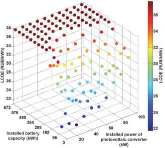
This problem is addressed using the coordinate descent method. The optimization algorithm involves a sequential search through the installed capacities of the system components. fig. 5 a and fig. 5 b show the optimization results and a diagram of the obtained solar radiation. The results indicate that the optimal technical configuration for the given consumer includes a solar power plant with an installed capacity of 30 kW, battery storage with a capacity of 96 kWh, and a diesel power plant with a capacity of 60 kW. This configuration yields a minimum LCOE of 21.7 RUB/kWh, with annual diesel fuel consumption of 19.5 metric tons. The annual energy production from the solar and diesel power plants is 40.6 thousand kWh and 92.1 thousand kWh, respectively. For this region, solar radiation was estimated using the method described in the paper. The highest values occur during the summer period (up to 200 kWh/m²), while the lowest values are observed in winter.

The modeling and optimization of the structure of the autonomous energy system were conducted using a typical meteorological year, with subsequent performance testing under extreme weather conditions. In particular, simulations of solar panel operation modes were performed with temperature effects taken into account, which significantly influence output voltage.

The modeling error was assessed using the original meteorological time series ts ₁ from the weather site, processed by linear interpolation to fill missing values and smooth anomalies, and compared to the same time series ts ₂ , processed using Service s 1. The results are presented in tab. 4, showing a notable improvement in modeling accuracy when using the s 1-processed data. These results demonstrate that the availability of reliable climatic data is a key factor influencing the accuracy of simulation and optimization of energy systems that incorporate renewable energy sources.

Tab. 4. Comparative analysis results

Time Series	Execution Time, s				Modeling Error, %
	D	M	P	Total	D	M	P
ts ^	72	121	3	196	15.5	18.5	22.9
tS2	58	122	3	183	5.0	6.3	8.6

Conclusion

a)

b)

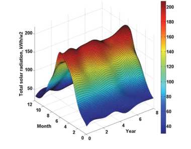
Fig. 5. Optimization of the structure and installed capacity of the energy system. (a) optimization results (b) solar radiation on the territory under consideration

The analysis of large-scale meteorological datasets and climate change information plays a vital role in addressing the challenges of rational environmental management, risk reduction from extreme weather events, and the effective management of nature-engineered systems in the socio-economic, technical, and industrial domains. However, such studies often require significant time and effort to collect and process meteorological data from open sources and to construct reliable models of meteorological years.

To this end, a service-oriented application has been developed as part of this research. The application integrates tools for retrieving, processing, and analyzing weather data. The services are implemented using the WPS standard, enabling their use in spatio-temporal data processing and environmental monitoring of natural areas. This application has been successfully applied to simulate the optimal structure of an autonomous energy system conditionally located in Eastern Siberia.

The application is implemented using modular service design principles, which ensures flexibility in updating and extending its set of services. The FDE-SWFs dispatcher interacts with the Kubernetes container orchestrator, enabling dynamic scaling of services based on the load across the nodes of the computing environment. A dedicated monitoring system integrated into the framework continuously tracks the performance and health of scalable services. It operates in conjunction with the Prometheus monitoring and instrumentation system.

Acknowledgements

The work was carried out within the framework of the grant № 075-15-2024-533 of the Ministry of Science and Higher Education of the Russian Federation for the implementation of a major scientific project on priority directions of scientific and technological development (reg. № 124052100088-3).