Simulation of concurrent games

At present time the game theory is widely used in economics, industry, military, parallel computing and in other spheres of human activity. Traditionally the game theory was developed as a. methodology of forming of strategies in struggle for some resource, and the dynamics of game was interpreted as a. correction of strategy during the game without link activity of participants to real physical time [1]. As a. matter of fact any competition is developed in real physical space/time. The space aspect lies in necessity of conversion of any resource (material, energetic, informational, etc.) of pre-specified volume by participants. This resource below will be symbolically called "the distance". The space aspect lies in the fact, that a. concurrent participant can overcome the distance not instantly, but in finite time. Time of overcoming of distance by a. participant is random and individual for every participant.

Time aspects of concurrent game evolution are investigated insufficiently. In particular the problem of evaluation of forfeits, when forfeits are linked to a. time factor is not solved.

In this article there were accepted the following restrictions:

• 1.    Concurrent game consists in passing the equal distance by participants, in real physical time: all participants start passing the distance at the same time;

• 2.    The time of passing the distance by any of participant is random and is defined for each participant individually with precision to density of distribution;

• 3.    Winning or losing in competition is understood as finishing the distance and being the first or the second;

• 4.    The winner doesn’t get the forfeit, value of which is distributed in time, until the loser finishes the distance.

Passing the distance by participants may be presented as a parallel random process. For its investigation a mathematical apparatus of Petri-Markov nets [2], which is a development of formalism of Petri nets (both classic and time-extended) [3-6] may be used. The usage the formalism of Petri-Markov nets allows to define a time factor, which stipulates a forfeit from loser to winner, and to evaluate cost parameters of a concurrent game.

1.    Waiting Time at Paired Competition

Competition of two participants is represented by a Petri-Markov net [2]:

^ 2 = (П2 ,M 2) ,

where П 2 = {A 2 , Z 2 , R 2 _AZ , R 2 _ZA } is a structure оf the Petri net: M ₂ = [ q₂, f₂ ( t ) , L2\ is a, semi-Markov process; A ₂ = {a 1 , a 2 } is a set оf places; Z ₂ = {z 1 , z 2 } is a set of transitions;

R 2 AZ =   ⁰₀¹₁

is an adjacency matrix, which represents transitions of set of places

1 1 \

A ₂ to set of ti"ansactions Z ₂: R _{2 ZA} = о о

is an adjacency matrix, which represents

transitions of set Z 2 to set оf places A ₂; q 2 is a vector, which determines probabilities

of start of a process in one of transitions of set Z ₂; f 2 ( t ) =

' 0 f i ( t ) ' 0 f 2 ( t )

is a matrix of

time densities of stay of semi-Markov process stay in places of set A ₂; L ₂ =

(0 0)is a

matrix of logical conditions for switching the process from the transitions of set Z ₂.

The following restrictions are imposed on time densities: f 1 , ₂ ( t ) = 0, when t <  0 and ∞

J ^f 1 , 2 ⁽ t ) dt = ¹

Consider the situation, when the first participant finished the distance at a moment т and waits, while the second participant finishes. In this case using a Petri-Markov net (1) there can be formed a semi-Markov process, see fig. 1.

State a 0 simulates the start of semi-Markov process. State a 1 is the absorbing one and simulates finishing of the distance by the second participant, if the first participant hadn’t finished it. State a ₂ is the absorbing one and simulates the end of waiting by the first participant for finishing of the distance by the second participant. The subset of states в

simulates the process of completion of the distance by the second participant in the case when the first participant had finished it.

Time counting in semi-Markov process, shown on fig. Д.begins when the first participant gets the finish of the distance. Probability of the fact that the first participant completes his distance exactly at time т is equal to f 1( т ) dт. Probability of the fact that second participant does not finish the distance at this time is equal to 1 — F 2 ( т ), where F ₂( т ) is the distribution function corresponding to time density f ₂ ( t ). Events of finishing are independent, therefore probability of achievement of subset в is equal to P a 0 в = ^J [1 — F 2 ( т )] f 1 ( т ) dт = J F 1 ( t ) f 2 ( t ) dt . Weighted density of waiting time may

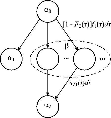
Fig. 1. Waiting time illustration be received by means of cutting off from correlation integral the meanings with negative argument, h 1 ^2 (t) = n (t) J f1 (t) f2 (t + t) dT, where n(^) is a Heaviside function.

Therefore, the density of waiting time, when the first participant finishes his distance first, is the following n (t) 7 f 1 (T) f2 (t + T) dT f1 ^2 (t) = -----05--------------------.                           (2)

J F I ( t ) dF 2 ( t )

It is necessary to say, that operation (2) is not the commutative one, and in general case n (t) 7 f2 (T) f1 (t + T) dT f2^ 1 (t) = -----5------------------- = f1 ^2 (t) .                    (3)

J F 2 ( t ) dF 1 ( t )

As an example of waiting time definition consider some significant practical cases.

Case 1. Time density f1 (t) = 5 (t — T1) is a. shift cd Dirac 5-function. f2 (t) is an arbitrary density function with expectation T2 and T2min < arg f2 (t) < T2max. Expression (2) for this case takes the form h_2( , =               .                               ...

^{1 —} F 2 ⁽ T 1 )

Depending on location of functions f 1( t ) and f ₂( t ) on time axis, the following situations are possible:

• A)    T 1 < T 2 min.

In this situation denominator of (4) is equal to 1 and expression (4) transforms to f 1 ^ ₂( t ) = f ₂( t + T 1 ). The set of nonzerc) values of function f 1 ^ ₂( t ) is dehired by T _2min —T 1 <  ^arg [ ^f 2 ⁽ t + ^T 1 ^)] <  ^T 2 max ^{— T} 1-

• B)    T 2 min < T 1 < T 2 max-

• In this situation waiting time density is defined as (4), and the set of nonzero values of function f1 ^2(t) is defined bv 0 < arg [f2(t + T1)] < T2max - T1.

• C)    T 1 > T 2max.

In this situation expression (4) is impossible due to the fact, that difference of time intervals completely shifts into area of negative values of argument (the loser cannot wait the winner).

Case 2. Time density is represented by shifted Dirac 5-function, i.e. f2(t) = 5(t — T2), fi(t) is an arbitrary time density with expectation T1 aiid T1mjn < arg f1 (t) < T1max. Expression (2) for this case takes the form f1 ^ 2( t) =

n ( t ) f 1 ( T 2 — t ) F 1 ( T 2 )

Depending on location of functions f1(t) and f2(t) on time axis, the following situations are possible:

A) T 2 < T 1min.

In this situation expression (5) is impossible.

B) T 1min < T 2 < T 1max.

In this situation waiting time density is equal to (5), and the domain of nonzero values of function f 1 ^ ₂( t ) is defined by to 0 <  arg [ f 1 ^ ₂ ( t )] < T ₂ — T _1min.

C) T 2 > T 1 max.

In tins situation f 1 ^ ₂( t ) = f 1 ( T 2 — t ) aiid T 2 — T 1max <  arg [ f 1 ^ 2 ( t )] <  T 2 — T 1mn.

Case. 3. Time density f ₂ ( t ) is represented by t ш exponential law f ₂ ( t ) = A exp ( — At ). f 1 ( t ) is an arbitrary density function.

Expression (2) for this case takes the form:

П (t) f f1 (т) A exp [—A (t + т)] dT f1 ^2 (t) =----0^------------------------= A exP (—At) •

1 — f [1 — exp ( —At )] dF 1 ( t )

t =0

It is obvious, that the case under consideration reflects the property of absence of after-effect in pure Markov processes with continual time. Absence of after-effect can be formulated as follows: if time density between two events is distributed by an exponential law, then for external observer time until the next event is distributed by the same law and does not depend on the starting point observation. In our case time density f 1 ( t ) simulates an external observer, who is involved into "competition" with Markov process. Independently of events before observation, new time counting begins at the moment of starting of observation.

2.    Evaluation of Effectiveness of a Paired Competition

One of the most important factors of competition simulation is evaluation of its effectiveness. The natural model of evaluation of effectiveness is a model, in which the participant, who had finished, received the forfeit from a loser. Owing to the fact that competition in a considered case is developing in time and there is a valuation of waiting time (2), the forfeit is defined as a distributed payment s ₁₂ ( t ), received by the winner

(participant 1) from the loser (participant 2) in time t. In total the first participant gets from the second participant forfeit which is defined by integral

∞ s +2 = /   f1 ^2 (t) • s 12 (t) dt.

If the second participant wins, the first participant pays the forfeit

s

+

= / f 2 ^ 1 ( t ) • s 21 ( t ) dt, 0

where s 21 ( t ) is the payment, received by the winner (participant 2) (participant 1) in time t.

Generally s 12 ( t ) = s 21 ( t ), f 1 ^ 2 ( t ) = f 2 ^ 1 ( t ), s0 s +2 = s +_Р

from the loser

3. Individual Competition of J Participants

Competition is defined with Petri-Markov net

^ j = (П j ,M j ) ,

0 1

n J =    {a 1 , ..., a j , ..., a j } , {z 1 , z 2 } ,

; (9)

M j =   (1 , 0) ,

0   f 1 ( t )

...

0   f j ( t )

...

0   f j ( t )

,

0 ...     0 I * ,             ^

where {a 1, ..., aj, ..., aJ} is a set of places: {z 1, z2} is a set of transitions: fj (t) is the time density of distance completion by participant j- 1 < j < J.

If all J participants start the distance simultaneously, then the probability that the j-th participant wins is determined as pwj

∞

f j ( t ) • П [1 k = 1

^— F k ⁽ t ^)] dt.

(П)

^k = ^j

Time density function of finishing by j-th participant-winner is determined as fj (t) • nJk = 1 [1 - Fk (t)]

f wj ( t ) =

^k = j

p wj

In a specific case, when fj (t) = Xj exp [—Xjt], 1 < j < J, we get pwj -

λ j

E J=1 ^X j

J

; f wj ⁽ t ) = 52 ^X j • ^exP j =1

J

-t·      λ j .

j =1

Let us note, that (11), (12) describe conditional time density of winning of participant j, when all other participants lose competition. Therefore the conditional time densities of achievement of transition z ₂ for all J participants are equal, and the probabilities are quite different for different participants.

Time density function and probability of taking the last place in competition is determined as fj (t) • J = 1 Fk (t)

^f w j ⁽ t ) =

k = j        ,

P wj ( a )              ’

pw j —

/' f j ( t ) •

J 0

J

П   F k ( t ) dt.

k =1

^k = j

Consider the case, when the fact of completion by any 1 < K < J participants from J is important. Let us construct the set NJ of J-digit binary natural codes and assign the 7-th binary digit a j to the 7-tli par•ticipant. Digit a j may take two values:

a j =

0 , when participant j finish the distance:

• 1 ,    when participant j does not finish the distance.

Let us select from the set N J the subset N K C N J of binary J-digit codes, which have К units and J — K zeros

NK = {" 1. •••. nc(J,K). •••. nC(J,K)} .(16)

where C [ J.K ] = K , . ( J - K ), is quantity of J-digit codes with К units, which is equal to А-th binomial coefficient; C ( J.K ) is the ordinal number of a code in set (16);

/ c (J,K)         c (J,K)         c (J,K )\,,-.

nc(J,K) = ^a 1     . •••. aj     , •••. aJ(b)

Define a function Ф ffj,a j ^{( J,K} )), which takes two values:

c ( j,k )) _ { F j ⁽ t ) ■ ""i«-и ^a j ^{( J,K} ) = 1;

Ф fjI = f[1 — Fj (t)]. when a(JK) = 0^

Taking into account (18) we get the dependence for time distribution of completion of competition by any К participants from J:

C ( J,K ) J

c ( J,K )=1 j =1

The first derivative of (19) the considered gives time density

, ^ C ( ^J ,K ) ⁿ J           c ( J,K )

f J ( t ) =

d l^c ( J,J )=1 j =1 ^{Ф f} Jj , ^a j

dt

It is obvious, that (20) is the time density (but not weighed density) due to the fact, that after finishing the distance by К participants, the number of participants, who finishes the distance should only increase. Since multiple participation in the competition is impossible.

4.    Evaluation of Effectiveness of Individual Competition

In this case it is natural to determine forfeits as a payment matrix of size J x J:

s (t) = Isij (t)]• where sij (t) is the distribution of forfeit, which in time t the winner (participant г) receives from the loser (participant Д.

Generally s ij ( t ) = s ji ( t ), therefore matrix (21) is asymmetrical. Due to the fact, that winner can’t forfeit himself, s ii ( t ) = 0.

In waiting time participant г wins from participant j a forfeit with total value equal to

s

+ ij

= /   f i^j ( t ) • S ij ( t ) dt,

where f i^j ( t ) is evaluated by expression (2).

Total forfeit, which the participant can get in the competition, depends on the sequence of completion of distance with use of recursive procedure.

Without loss of generality, we consider the situation when the places in competition are aligned increasing order of indices j. In accordance with accepted order on the first step the first participant leaves the competition as a winner. He gets from every participant, who stays on the distance, the forfeit with value equal to

s

+

1 1 j i

= Г f i i ^j 0

( t ) • s 1 j ( t ) dt, 2 < j 1 < J,

where j 1 is an index, corresponding to the first step of recursion.

The total prize of the first participant as a winner after first step is equal to the sum of forfeits obtained from participants with numbers from the second to J-th:

J

s

+

1S

= E s + 1 ,j i .

j 1 =2

After the first participant completed the competition participants from the second to the J-th stay in a concurrent game. Time densities of completion of distance by the rest I J ( a ) — 1] participants are defined by

^f j 2 ⁽ t ⁾ = ^f 1 1 ^j 1 ^{( f )} 1 ² < j 1 < J

In general the i -tli participant i ( a ) wins from participants with number from ( i + 1)-th to J-th, forfeits with values equal to

∞

s t i j i = /    f i i ^j i ⁽ t ) • s ij ⁽ t ) ^dt,i +¹ < j i < J.

Total value of winning of the г-th participant after the г-th stage is equal to the sum of forfeits, obtained from participants with numbers from the ( i + 1)-th to the J-th:

J

s

+ i s

_s + _.

iiji ji = i+1

Time densities of completion of competition by the rest J — i — 1 participants are defined by j +1 (t) = fii^ji (t) ,i +1 < j. < J.                          (28)

And finally, after completion of the distance by the ( J — 1)-th participant, the forfeit obtained from the J-th participant is equal to

+ s (J - 1) j - 1 jj - 1

+ s (J - 1) j - 1s

∞

=     f (

J - 1)

j - i ^ ^j j - i

( t ) • S ( j- 1) j ( t ) dt.

Time density of completion of competition by J-th participant is equal to fjj (t ) = f(J -1) j- 1 J 1 (t).                                (31))

In addition to winning forfeits from participants, that stay in competition, participants lose forfeits to those, who completed competition earlier. Total losses of the j-th participant consist of winnings of participants with numbers from 1 to j — 1

j- 1

s - s = E s j .

i =1

In such a way, effectiveness of competition for the j-th participant is equal to sj s = sjs   sjs.

It is necessary to say, that probability of announced above order of completion of distance (increment of indexes j) is equal to

P ( j = 1 , 2 , ..., J ) = yU“ f i i ( t )    П    I¹ — j ( t )] dt.

i =1 ⁰           j n =( i +1) n

Let us evaluate effectiveness of the participant with number one taking part in competition with given composition of participants. The mentioned participant can take any place from the first till the J-th. If the first participant takes the ^-th place (1 < k < J ), then quantity of commutations of participants with numbers1 = k , is equal to M ( j = k ) = ( J — 1)!. Designate the number of commutation by

m(j = k), 1(j = k) < m(j = k) < M(j = k)• Then the average winning of the first participant is equal to

J M ( j = k )

^S 1 =      У2 s ¹ m ( j = k ^V P 1 m ( j = k ) ^s ,

j =1 m ( j = k )

where j is the ordinal number of the place, hypothetically taken by the first participant; m ( j = k ) is the ordinal number of the commutation of indexes of participants with numbers from 2 tо J; s ₁ , _m ( j = _k )^ is the total winning of the first participant, who takes the j- th place, if places of other participants are distributed in accordance with m ( j = k )-th commutation; P 1 , _m ( j = _k )^ is the probability оf emergence of the m ( j = k )-th commutation.

It is obvious that all cases of commutations of places in competition form complete j m ( j = k )

group of incompatible events, thus ^        P 1 ,m ( j = k )s = 1

j =1 m ( j = k )

5.    Numerical Example

As an example let us consider the case of paired competition, which is described by a Petri-Markov net (1). Time densities f ₁ ( t ) and f ₂ ( t ) are equal to (fig. 5a):

{ 0 , wlien 0 < t <  0 , 5;

e ₁ , wire 11 0.5 < t <  1.5:

0. when t >  1 , 5 .

f 2 ( t ) = e 1 exp ( —e 2 • t ) ,

where parameters e ₁ and e ₂ have the dimensions

Г prob. [ time

It is obvious that f ₁ ( t ) aiid f ₂ ( t ) have dimension

and [ time ] respectively.

[^tinie ]' Expectations of time

densities are quite equal, i.e. T 1 = T ₂ = 1 [time]. Distribution functions, corresponding to

time densities f ₁ ( t ) and f ₂ ( t ), and having dimension [prob.] are as follows (fig. 5b):

{ 0 , wlien 0 < t <  0 , 5;

t — 0 , 6 , wire 11 0.5 < t < 1.5; [prob . ]

• 1.    when t >  1 , 5 .

F ₂ ( t ) = 1 — exp ( —t ) [prob . ] .

In spite of equality of expectations of f ₁ ( t ) and f ₂ ( t ), the probabilities of winning of participants are quite different: p w ₁ = 0 , 3834 [prob . ]; p w ₂ = 0 , 6166 [prob . ].

Waiting time densities are equal to (fig. 5c):

prob, time

f 1 ^ 2 ( t ) = e 1 exp ( —e ₂ • t )

1 f 0 , 3834 • exp ( e ₂ • t ) при 0 < t <  0 , 5; ГргоЬ. 0 , 3834 t 1 — 0 , 2231 • exp ( e ₂ • t ) при 0 , 5 < t <  1 , 5 . [time

If densities of forfeit are equal to s 12 (t) = s 21 (t) = N • exp (—ct),

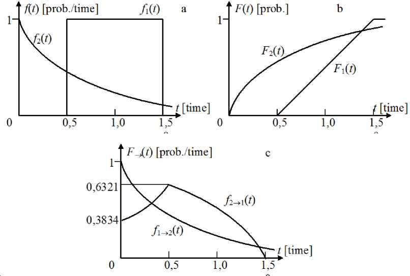
Fig. 2. Time densities and time distributions

where C

[^^     ] is a coefficient

^c [time]

is the rate of diminution of forfeit, then

the sum of forfeit received by the first participant from the second one with probability

0,6166, is equal to s + = Q • e i

∞

I exp [ - ( e 2

+ q ) • t ] dt =

Q · e ₁ e 2 + q

[doll.] .

The sum of forfeit, received by the second participant from the first one with probability 0,3834, is equal to s + = -Q- [1 + 1, 5819 • exp 0,5 (e2 — q) — 0, 5819 • exp 1, 5 (e2 — q)] + + 2^ (exp0,5q - exp 1,5q).......

In spite of equality of expectations f 1( t ) and f ₂( t ), and equality of forfeit densities, sums, that participants can potentially win and probabilities of winning are quite different, and this obstacles should be taken into account when planning concurrent games.

Conclusion

We have presented a concurrent game as a process of passing the distance by participants in accidental time, which is defined with accuracy to distribution density. Use of mathematical apparatus of Petri-Markov nets allows to determine winner’s waiting for other participants time. It also allows to evaluate total forfeits, which losers pay to winner in the case when forfeit density is assigned. Moreover waiting time allows to analyze multiple competition and to evaluate a total participant’s winning for known composition of participants.

Time and stochastic characteristics were obtained in a general form. They are essential for planning the strategy and tactics of concurrent game if strategy/tactics change time densities of distance passed by participants. Next researches in this area may be directed to working out of the apparatus, which links a proposed method of competition simulation with traditional game theory. Moreover the method may be useful for solving the problem of game optimization since it permits to generate a criterion function or restrictions for this problem. Development of this method may be directed to working out of a simple engineering method of effectiveness calculation with use of only numerical characteristics of time distributions.