Soft Attention Enhanced CNN and LSTM Based Framework for Semantic Description Generation of Remote Sensing Imagery

Published Online on August 8, 2026 by MECS Press

One of the key applications of Intelligent systems is generating appropriate description for an image. Many attempts have been made to develop an intelligent image description generator capable of producing human-like narratives; still, it remains a challenge[1, 2, 3]. Especially in the case of remote sensing images, generating contextual semantic image descriptions poses significant challenges due to the heterogeneous and complicated scenes[4]. Remote sensing images often contain varied landscapes with similar spectral appearances and mostly contain multiple objects leading to ambiguity in interpretation. Accurate identification of the relevant features and understanding the contextual relationships between them is a complicated task in the case of remote sensing images. Moreover, the lack of well-defined object boundaries and the presence of noise or low-resolution areas further complicate the task. These factors make it challenging for models to generate precise and semantically correct descriptions.

The recent description generation applications are empowered by the advances in the fields of remote sensing image processing and natural language processing, yet there is a common argument about the applicability of these systems, as humans can examine and describe images faster and more accurately than computers. The system generates descriptions of remote sensing images through several tasks. These tasks involve detecting objects, understanding the context, predicting the relationships between the objects and their environment, and creating grammatically and semantically correct descriptions for each image[5]. The task of description generation poses a real challenge while dealing with large volumes of image. For instance, in applications for analyzing satellite imagery, for thousands of images, a detailed description is required to extract valuable insights. Manually drafting the descriptions would be a time-consuming and tiresome task. In such cases, automated image description systems can quickly generate descriptions. For good analysis, it is important to generate the description that covers all the aspects of the information present in the remote sensing image and generate meaningful, unambiguous sentences. Despite significant advances in remote sensing image description generation, existing methods face several limitations in complex remote sensing scenarios. Conventional CNN–LSTM encoder–decoder architectures primarily rely on globally extracted visual features and may fail to selectively emphasize spatially relevant image content during word generation[6, 7]. Recent multiscale attention and Transformer-based architectures improve feature interaction and long-range dependency modelling; however, their architectural complexity can impose substantial computational requirements. Moreover, till date efficiently capturing fine-grained structural information and achieving effective visual–linguistic alignment remains challenging in heterogeneous remote sensing scenes[8, 9, 10]. Furthermore, the performance of description generation architectures is often evaluated on individual benchmark datasets, providing limited evidence of their robustness across datasets with varying spatial resolution, scene complexity, and object distribution. This research gap motivated to perform a study with the objective to systematically examine whether a computationally simpler attention-enhanced CNN–LSTM architecture can improve visual–linguistic alignment and semantic description quality while maintaining consistent performance across heterogeneous remote sensing datasets. The proposed framework dynamically aligns the decoder hidden state with encoded visual features to selectively emphasize contextually relevant image information during word generation. Unlike conventional CNN–LSTM architectures based primarily on global feature representations, the attention-guided decoder explicitly integrates visual relevance with linguistic context. The study further conducts a comparative evaluation of multiple CNN encoders with and without attention and assesses the robustness of the best-performing architecture across the UCM, RSCID, and Sydney Caption datasets. The major contributions of this study include

• •    Development of a soft-attention-enhanced CNN–LSTM framework that dynamically integrates encoded visual information with the decoder hidden state for remote sensing image description generation.

• •    Systematic comparative assessment of five CNN feature extractors (VGG16, VGG19, Inception, ResNet50, and ResNet152) with LSTM decoders under attention and non-attention configurations using BLEU-1 to BLEU-4 metrics and qualitative human evaluation of accuracy, completeness, grammatical correctness, and semantic correctness.

2.    Literature Survey 3.    Methodology

The subject of remote sensing image description generation has made remarkable progress recently. Researchers have investigated a variety of ways to generate descriptions for remote sensing data, addressing issues such as change detection, context comprehension, and varied object recognition.

The basic encoder-decoder-based architecture depends on neural network topologies that lack specialized capabilities for selecting and concentrating on certain portions of an image during the description-generating process. Vinyals et al. [7] recommend a neural and probabilistic framework for generating remote sensing image descriptions, leveraging recent advancements in statistical machine translation. They propose a model coupled with a CNN and LSTM network for sentence generation. BLEU score is used as an evaluation metric to assess the performance of the proposed model on datasets such as Pascal VOC 2008, Flickr8k, Flickr30k, MSCOCO, and SBU. Shi et al. [11] developed a deep learning-based model that demonstrates strong transferability and effectiveness for generating the description for images from Google Earth and the GaoFen-2 satellite images. Unlike previous approaches, they employ a subjective evaluation criterion rather than objective methods like BLEU or ROUGE. Huang et al. [12] introduced a novel Denoising-Based Multiscale Feature Fusion (DMSFF) mechanism for improving remote sensing image captioning. To address the large-scale variations in remote sensing images, model discussed in this study integrates denoising operations with feature extraction. This enhanced the encoder-decoder framework's ability to generate accurate and comprehensive captions. Mao et al. [13] discussed a Multimodal Recurrent Neural Network (m-RNN) model for image caption generation which is a combination of deep RNN and deep CNN models. These two subnetworks interact with each other for sentence modelling. The performance evaluation of m-RNN is conducted on benchmark datasets including IAPR TC-12, Flickr 8K, Flickr 30K, and MS COCO where m-RNN demonstrated state-of-the-art performance in sentence generation. Even though deep learning models are widely used, Hoxha et al. [14] address the challenge of generating captions for remote sensing images using a network of support vector machines (SVMs). This approach comprises a pre-trained ResNet50 model to extract visual features from images, which are then processed by a cascade of SVM classifiers to generate textual descriptions. This architecture is validated on a UAV-acquired remote sensing image dataset, demonstrating promising results with BLEU scores outperforming a multimodal RNN model in certain metrics. It comes up as a viable method for remote sensing image description generation when limited annotated samples are available. Sumbul et al. [15] introduce an approach that addresses redundancy and vocabulary limitations in existing datasets. Their approach consists of standard caption generation using CNN-LSTM, ground-truth caption summarization, and adaptive integration of summarized and standard descriptions. Evaluation on established datasets like Sydney-Captions, UCM-Captions, and RSIC demonstrates the efficiency of this approach, with improvements attributed to redundancy elimination, vocabulary enrichment, and adaptive weight integration. To address the challenges in description generation due to the complexity of remote sensing images, Wang et al. [16] presented a model that leverages semantic embedding and metric learning to generate descriptive text. Lu et al. [17] suggested a sound-active attention framework for high-resolution remote sensing image captioning, allowing for descriptive sentence generation based on both image content and accompanying sound cues. Here a CNN is used as a feature extractor for visual information, sound cues are integrated through sound-active attention mechanisms, and a description decoder is used for description generation. Wu et al. [18] propose a model that combines CNN feature extraction with LSTM and introduces scene attention to leverage global visual information and current hidden states for better focus on relevant scene elements. In another study, Chen et al. [19] explore a novel spatial-temporal attention neural network for binary remote sensing image change detection, accompanied by the creation of a substantially larger dataset called LEVIR-CD. This model comprised of the Pyramid Spatial-Temporal Attention Modules to capture spatial-temporal dependencies by mitigating misregistration issues and enhancing robustness to color and scale variations. This approach outperforms state-of-the-art methods on the SZTAKI dataset and offers potential for integration with Siamese-FCN-based CD algorithms. Zia et al. [20] created a groundbreaking encoder-decoder architecture for describing remote sensing images. It has a multi-scale visual feature extractor and an adaptive multihead attention decoder. The Multi-Scale Adaptive Attention (MSAA) mechanism dynamically assigns weights to multiscale features and textual cues, facilitating the contextually rich description. This unique model not only enhances the description quality but also addresses the challenge of large variances in visual aspects. Another research carried out by Zhang et al. [21] suggested a novel framework combining the global visual feature-guided attention (GVFGA) and linguistic state-guided attention (LSGA) mechanisms to enhance remote sensing image captioning. The GVFGA mechanism fuses and refines global and local image features, while the LSGA mechanism extends the LSTM network to fuse visual and textual features, filtering out redundant information.

Transformers have gained popularity owing to their capacity to capture long-term dependencies and linkages in sequential data, making them ideal for acquiring spatial and temporal knowledge. Unlike traditional approaches, Chen et al. [22] proposed a transformer-based framework with a PViT-b5 encoder that effectively captures multiscale object information using a vision transformer and generates user-oriented descriptions by embedding required caption through the caption-type controller. This model is evaluated on the RSICD and FloodNet datasets, showcasing its capability to generate accurate and diverse description tailored to specific types of remote sensing images. To enhance feature discrimination Liu et al. [23] uses a combination of a CNN, a dual-branch Transformer encoder (DTE), and a description decoder. To address the challenge of limited training data, Kandala et al. [24] discuss a transformer-based framework, augmented with an auxiliary LSTM-based decoder. The proposed model demonstrated its effectiveness in generating coherent textual descriptions for remote sensing images. Sen He et al. [25] introduce the image transformer architecture, widening transformer layers to adapt to the image structure. Their model leverages spatial relationships between image regions in both the encoding and decoding stages, trained on Visual Genome data using Faster R-CNN.

Table 1 presents a comprehensive overview of the of the existing literature. Although transformer-based and attention-based architectures demonstrate substantial performance in remote sensing image description generation, still significant challenges persist. In particular, efficiently modelling relationships among objects and integrating semantic

Table 1. Literature Overview.

Author Dataset Preprocessing Methodology Chen et al. [22] RSICD, Floodnet - Transformer architecture for image representation, breaking down images into patches and multihead self-attention layers to capture both fine-grained and coarse-grained features at different scales. Liu et al. [23] LEVIR-CC - CNN, a dual-branch transformer encoder, and a caption decoder Kandala et al. [24] UCM Captions - Transformer encoder-decoder architecture with an auxiliary LSTM-based decoder for multilabel classification Sen He et al. [25] MSCOCO Discarding the words that occurs less than 4 times before creating a vocabulary Image Transformer fuses encoding and decoding transformers to handle spatial relationships and diverse image region information. Vinyals et al. [7] Pascal VOC 2008, Flickr8k, Flickr30k, MSCOCO, and SBU Tokenization and discarding the words that occur less than 5 times before creating a vocabulary. CNN coupled with a language-generating RNN Shi et al. [11] GaoFen-2 satellite and Google Earth images Images are cropped, converted to 8-bit using ENVI software, and ambiguous instances without bounding boxes are discarded. A two-stage approach: First, a single FCN model detects and identifies ground elements; second, language generation stage. Huang et al. [12] UCM captions, and Sydney captions Resizing and horizontally flipping DMSFF mechanism. Mao et al., [13] IAPR TC-12, Flickr 8K, Flickr 30K, and MS COCO - m-RNN model Hoxha et al. [14] Images taken by UAV using an EOS 550D camera near Civezzano city, Italy Generated a non-overlapping frames dataset with each image resolution 256 × 256. A Pre-trained CNN and a network of SVMs Sumbul et al. [15] RSCID, UCM captions, and Sydney captions datasets In cases with fewer than five captions, captions were augmented by randomly duplicating existing ones. The SD-RSIC approach comprises three key steps: generating standard captions using CNN-LSTM, summarizing ground-truth captions, and integrating these summaries with standard captions. Wang et al. [16] RSCID, UCM captions, and Sydney captions datasets - Proposed Collective Semantic Metric Learning Framework Lu et al. [17] UCM captions, Sydney captions, and RSICD MFCCs for sound modeling and CNNs for image encoding MFCC-based sound modelling with CNN-based image encoding and GRU-based sound and attention modules to maintain sound continuity Wu et al. [18] UCM captions, Sydney captions, and RSICD datasets - The scene attention mechanism combines LSTM's current attention with global visual information derived from the mean of all convolutional features. Chen et al. [19] SZTAKI, OSCD, Aerial Imagery Change Detection dataset, and LEVIR-CD Subregion partitioning Utilizes Siamese architecture with CD self-attention for remote sensing change detection. Zia et al. [20] RSICD, UCM captions, and Sydney captions - The proposed model excels with adaptive attention, multi-scale features, and topic-sensitive word embedding in benchmarks. Zhang et al., [21] RSICD, UCM captions, and Sydney captions - The model uses adaptive attention and multi-scale features to improve remote sensing image captions, showing promising results in benchmark datasets. and syntactic information remain challenging. To address these limitations, this study investigates a soft attention enhanced encoder–decoder architecture to generate description efficiently. The detailed discussion on the proposed framework architecture is carried out in section 3. The performance of the evaluated architectures is discussed in Section 4. Furthermore, the best-performing architecture is compared with existing approaches and demonstrates superior performance in terms of BLEU score.

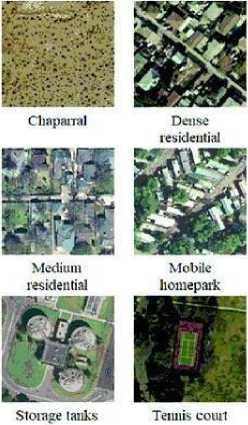
The proposed work uses the UC Merced dataset. The UCM dataset comprises 21 classes of land use, each with 100 images. The dataset encompasses diverse urban areas nationwide, featuring classes such as runway, agricultural, intersection, dense residential, airplane, medium residential, baseball, overpass, beach, buildings, chaparral, forest, freeway, golf course, harbor, mobile home park, parking lot, river, sparse residential, storage tanks, and tennis court. Although most images are 256x256 pixels, 44 images deviate from this shape [26]. Figure 1 shows sample images from different classes of the UC Merced dataset. The model performance robustness is tested on the other benching datasets like RSCID and Sydney captions to provide a good model. The RSCID dataset comprises a total of 10,921 images with 224 × 224 pixel resolution. These images are categorized into 30 classes, and each image has five captions. RSCID is considered as one of the largest datasets used for remote sensing image caption generation task. On the other hand, the Sydney Captions dataset contains a total of 613 images with 500 × 500 pixel resolution. These images are categorized in 7 classes and have five captions per image.

Agricultural            Airplane             Baseball              Beach              Buildings diamond

Forest             Freeway          Golf course           Harbor           Intel section

Overpass          Parking lot           River            Runway            Sparse residential

Fig. 1. Dataset overview.

The UCM dataset was randomly divided into training (80%) and testing (20%) subsets while preserving class balance. The same partitioning strategy was adopted for the RSCID and Sydney Caption datasets. Random shuffling was performed before partitioning using a fixed random seed to ensure reproducibility. All reported results were obtained using identical dataset partitions across all evaluated models.

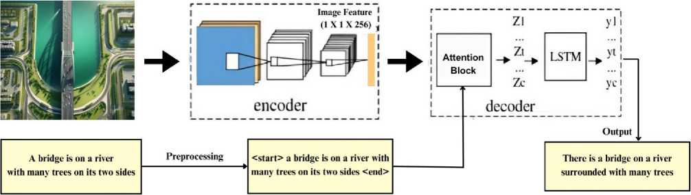
Fig. 2. System Architecture.

Figure 2 gives an overview of system architecture. It comprises an end-to-end encoder-decoder model with an attention mechanism for generating semantic descriptions of remote sensing images. It involves two main elements:

• a.    Encoder or feature extraction model.

• b.    Decoder or language model with attention model.

• 3.1.    Encoder

• 3.2.    Decoder

A deep neural network, CNN, is used as a feature extraction sub-model. It is capable of extracting the salient features from the given image in the form of a fixed-length vector. We experimented with ResNet50, ResNet152 [27], Inception [28], and VGG16 and VGG19 [29], popular convolutional neural network architectures, to extract meaningful and discriminative features from the input image [30]. Here, VGG16 has shown prominent results; hence, the feature extraction process using the VGG-16 architecture [31] is elaborated in depth. VGG16 is a widely used convolutional neural network architecture known for its uniform stack of small (3×3) convolutional filters arranged in depth, which allows it to learn increasingly abstract visual features through depth alone, without residual or skip connections. The 224x224 pixel input image with three RGB color channels is convolutionally processed by VGG-16. The 224x224 pixel input image with three RGB color channels is convolutionally processed by VGG-16. The layers use filters to identify various visual features such as edges and textures.

Unlike ResNet-50, VGG-16 does not use residual blocks; instead, it stacks convolutional layers and applies maxpooling for spatial reduction. Toward the end, a flatten layer followed by the dense layers is applied, which collapses spatial dimensions into a fixed-length feature vector, usually 4096 in dimension. The last two layers of VGG16 generally used for classification are removed. Thus, the final output is a 4096-dimensional feature vector that captures important visual information. To reduce overfitting, a dropout layer is introduced. During each training iteration, a fraction of neurons is randomly dropped during the dropout layer. This allows the model to avoid over-reliance on particular neurons, resulting in a more diverse representation. Moreover, the dropout layer improves the model’s generalization to unseen data through the introduction of a form of normalization during training. The dropout operation is implemented as element-wise multiplication of the 4096-dimensional feature vector (output of the fc2 layer) with a binary mask whose entries are drawn from a Bernoulli distribution, with a dropout rate of 0.5. A dense layer is incorporated immediately after the dropout layer. The output of the dense layer can be represented by equation 1.

Dense_output = ReLU(Dropout(Input) × Weight + Bias)                      (1)

Where, Input e R4096 denotes the 4096-dimensional feature vector from VGG16's fc2 layer. Weights e R4096x256 and Bias e R256 represents the learnable parameters of the dense layer. Dropout denotes the dropout operation. ReLU is the Rectified Linear Unit activation function. Dense_output e R256 subsequently referred to as Encoder_output.

This layer, which has an output size of 256, deftly extracts and summarizes the most important relationships present in the feature vector. It is represented as Encoder_output. This subtle transformation was made possible by the layer's learnable parameters and ReLU activation function, which allowed the model to provide meaningful representations that supported the next phases in the semantic description generation process.

The LSTM network is commonly used language model suitable for sequence prediction problems like description generation [32, 33]. For this study, LSTM is used to generate image description based on the combination of image features and textual context. Moreover, an attention mechanism is introduced to dynamically weight the importance of different parts of the input image during the semantic description generation process [34]. During the model training process, the tokenized description serves as a complementary input alongside other primary inputs, i.e., image feature vectors. The model is trained to understand the relationships between images and their associated tokenized descriptions, enabling it to make meaningful predictions. An embedding layer transforms the words from the input caption (input_2) into dense vectors. The transformation can be stated mathematically as shown in equation 2.

Embedding (Input_captions) = Embedding_output                         (2)

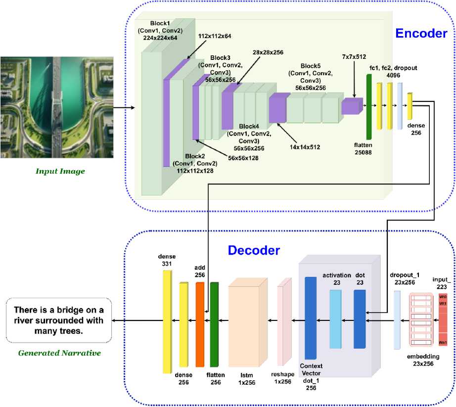
Fig. 3. Overview of the model.

The word order that was entered for the description is represented by the variable input_captions, and the output after embedding process is represented as embedding. In a continuous vector space, every word is uniquely represented by a vector of 256 dimensions; this dimension was chosen to match the encoder's output dimension (256), enabling direct element-wise fusion later in the decoder without a separate projection layer. The embedded sequence, of shape (23, 256) for a maximum description length of 23, is then passed through a dropout layer (rate 0.5) before being used in the attention step. By making it easier to capture the semantic ties between words, this mapping helps the model discover meaningful relationships between various keywords. For rich representations of the input description, the resulting dense vectors is given to the model to understand and extract meaning from the textual data. The attention weights were computed as the dot-product similarity between the encoder's output (a global 256-dimensional image feature vector, acting as the query) and each time step of the embedded description sequence (acting as the keys), producing one similarity score per description position. Mathematically, this operation can be expressed by equation 3.

Att_weight = Softmax(Encoder_output ∙ EncBits) (3)

Here, Encoder_output e R256 denotes the feature vector from the encoder. Embedding_output e R23x256 denotes the embedded (and dropout-regularized) description sequence. The dot product is taken along the shared 256dimensional feature axis, producing Att_weights e R23, one score per description position.

Subsequently, the attention weights were multiplied with the embedded description sequence, resulting in a weighted sum that represented the context vector. Mathematically, the context vector (Context_vector e R256.) is represented by equation 4. This process is illustrated in figure 3 as the dot, activation, and dot_1 layers, which take the encoder’s dense output and the description’s dropout_1 output as inputs which is consistent with the computation shown in Eq. 3-4.

Context_Vector = Att_weight ∙ Embedding_output (4)

The context vector (Context_vector) passes through the reshape layer to reshape the tensor shape of (None, 256) into (None, 1, 256), because the subsequent LSTM layer requires a 3-dimensional input of the form (batch, timesteps, features); the context vector is treated as a single-timestep sequence. The reshaping operation doesn't alter the information content of the tensor but introduces a new dimension. The reshaped vector is then passed through an LSTM layer [33]. The LSTM is designed to work with sequences and capture temporal dependencies. The LSTM layer consists of multiple units (256 units in this case), each equipped with various gates and hidden states. The output of an LSTM layer is passed through a flatten layer, thus transitioning it from a sequence data representation to a flat, onedimensional vector of size (None, 256) represented as flattened_LSTM_output. The output of the flatten layer (flattened_LSTM_output e R256) and the output of the encoder (Encoder_output e R256) share the same dimensionality and are combined through element-wise addition. This fusion operation merges the textual information generated by the LSTM with the visual features of the image. The resulting fused vector (fusion_result), obtained via element-wise addition, was used as input for the subsequent layers in the decoder, furnishing a refined, context-aware representation for generating the next word in the description. It enables the model to incorporate both visual and linguistic cues into the description generation process, enhancing the richness and contextuality of the generated narratives. This layer is represented by equation 5.

Fitting _ Result = Encoder _output + flattened_LSTM_output (5)

The image-text fusion generates fused features are processed further through a fully connected layer. This dense layer contains 256 neurons and applies the ReLU activation function. This step refines the combined features, allowing the model to capture more intricate relationships between the visual and textual components. The processed features from the previous step are fed into the final dense layer, followed by a SoftMax activation function. This output layer represented by equation 6, produces a probability distribution over the vocabulary of words. Each value in the distribution represents the likelihood of a specific word being the next word in the description narratives sequence. The word with the highest probability is predicted to be the next. This comprehensive approach enhances the quality of the generated descriptions for your remote sensing images.

predicted_probs = softmsx(W output ∗ output_FC + b_output) (6)

where, output_FC e R256 denotes output of the fully connected layer. W_output e W ^{0 cab} - ^slze and b_output e R ^_ represents weights and biases of the output layer. predicted_probs ∈ R ^_ denotes probability distribution over the vocabulary. _ denotes the predicted probabilities over the vocabulary and Softmax is the activation function.

Table 2. Layers of the Model.

Layer (Type)	Output Shape	Number of Parameters	Layer (Type)	Output Shape	Number of Parameters
Encoder			Decoder
input_1 (InputLayer)	[(None, 224, 224, 3)]	0	Input_2 (InputLayer)	[(None, 23)]	0
block1_conv1 (Conv2D)	(None, 224, 224, 64)	1792	embedding (Embedding)	(None, 23, 256)	84736
block1_conv2 (Conv2D)	(None, 224, 224, 64)	36928	dropout_1 (Dropout)	(None, 23, 256)	0
block1_pool(MaxPooling2D)	(None, 112, 112, 64)	0	dot (Dot)	(None, 23)	0
block2_conv1 (Conv2D)	(None, 112, 112, 128)	73856	activation (Activation)	(None, 23)	0
block2_conv2 (Conv2D)	(None, 112, 112, 128)	147584	dot_1 (Dot)	(None, 256)	0
block2_pool(MaxPooling2D)	(None, 56, 56, 128)	0	reshape (Reshape)	(None, 1, 256)	0
block3_conv1 (Conv2D)	(None, 56, 56, 256)	295168	lstm (LSTM)	(None, 1, 256)	525312
block3_conv2 (Conv2D)	(None, 56, 56, 256)	590080	flatten (Flatten)	(None, 256)	0
block3_conv3 (Conv2D)	(None, 56, 56, 256)	590080	add (Add)	(None, 256)	0
block3_pool(MaxPooling2D)	(None, 28, 28, 256)	0	dense_1 (Dense_1)	(None, 256)	65792
block4_conv1 (Conv2D)	(None, 28, 28, 512)	1180160	dense_2 (Dense_2)	(None, 331)	85067
block4_conv2 (Conv2D)	(None, 28, 28, 512)	2359808
block4_conv3 (Conv2D)	(None, 28, 28, 512)	2359808
block4_pool(MaxPooling2D)	(None, 14, 14, 512)	0
block5_conv1 (Conv2D)	(None, 14, 14, 512)	2359808
block5_conv2 (Conv2D)	(None, 14, 14, 512)	2359808
block5_conv3 (Conv2D)	(None, 14, 14, 512)	2359808
block5_pool(MaxPooling2D)	(None, 7, 7, 512)	0
flatten (Flatten)	(None, 25088)	0
fc1 (Dense)	(None, 4096)	102764544
fc2 (Dense)	(None, 4096)	16781312
dropout (Dropout)	(None, 4096)	0
dense (Dense)	(None, 256)	1048832

Figure 3 gives an overview of the framework used to generate the description. Table 2 represents the layer-wise number of parameters of the proposed model. Table 3 represents the key hyperparameters used across all trained models.

Table 3. Model Hyperparameters.

Hyperparameter	Value	Hyperparameter	Value
Dropout rate	0.5	Optimizer	Adam
Embedding dimension	256	Learning rates evaluated	0.0001, 0.001
LSTM units	256	Train/test split	80% / 20%

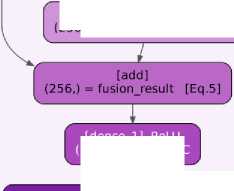
Figure 4 summarizes the complete forward pass by tracing the tensor shape at every stage of the encoder, attention block, and decoder, using the same variable names introduced in equation 1 –6, to further support reproducibility, Algorithm 1 formalizes the forward pass as pseudocode, and Algorithm 2 describes the autoregressive procedure used to generate a description at inference time.

Input image [input_l]

(224,224,3)

lnput_captions [input_2] (maxlength,)

VGG16 Blocks 1-5 [blockl_convl...block5_pool]

(7,7,512)

[embedding] (maxjength,256)

[dropout l] rate-0.5

(maxjength,256) = Embedding_output [Eq.2]

Encoder (VGG 16) - Table 2

[fcl] -> [fc2] (4096,)

[dropout] rate=0.5 (4096,)

key IK)

[dense] ReLU

»,) = Encoder output [Eq.l]

query (Q)

ition (Eq. 3-4)

[dot] Q.K^T = dot(Encoder output, Embeddingoutpuf^T) (maxjength,)

[activation] Softmax (maxjength,) = Attweights [Eq.3]

value (V)

[dot_l] weights.v = dot(Attweights’"T, Embedding_output) (256,) = Context vector [Eq.4]

[reshape] [256,) -> (1,256)

[Istm] units=256

(1,256)

[flatten]

[256,) = flattened J-STM_output

(dense 1] ReLU (256,) = output_FC

[dense_2] Softmax (vocab_size,) = predictedprobs [Eq.6]

Fig. 4. Tensor dimension flow diagram.

Algorithm 1. Forward pass of the proposed model

Require: image I (224×224×3), description token sequence C (length max_length )

Ensure: predicted_probs , a probability distribution over the vocabulary

// Encoder

1: F_vgg ← VGG16_ConvBlocks( I )	shape (7,7,512)
2: F_flat ← Flatten( F_vgg )	shape (25088,)
3: F_fc ← FC2(FC1( F_flat ))	shape (4096,)
4: F_drop ← Dropout( F_fc , rate=0.5)	shape (4096,)
5: Encoder_output ← ReLU(Dense 256 ( F_drop )) // Description embedding branch	shape (256,) — Eq. 1
6: E ← Embedding( C )	shape (max_length,256)
7:    Embedding_output ← Dropout( E , rate=0.5) // Attention block 8:    scores ← Encoder_output · Embedding_output ᵀ	Eq. 2
9: Att_weights ← Softmax( scores )	Eq. 3
10:    Context_vector ← Att_weights ᵀ · Embedding_output // Decoder tail 11:    Context_reshaped ← Reshape( Context_vector , (1,256)) 12:    LSTM_out ← LSTM 256 ( Context_reshaped ) 13:    flattened_LSTM_output ← Flatten( LSTM_out )	Eq. 4
14:    fusion_result ← Encoder_output + flattened_LSTM_output 15:    output_FC ← ReLU(Dense 256 ( fusion_result ))	Eq. 5
16:    predicted_probs ← Softmax(Dense vocab ( output_FC )) 17:    return predicted_probs	Eq. 6

Algorithm 2. Description generation (inference loop)

Require: photo_feature (4096,), a precomputed VGG16 feature vector for image I ; tokenizer , max_length , vocab

Ensure: generated description (string)

1: in_text ← “startseq”

2:    for i = 1 to max_length do 3:    sequence ← Tokenize( in_text ) 4:    sequence ← Pad( sequence , length= max_length ) 5:    predicted_probs ← ForwardPass( photo_feature , sequence ) 6:    next_id ← argmax( predicted_probs ) 7:    word ← WordForId( next_id , tokenizer )	integer-encode description so far Algorithm 1, lines 6–17 greedy decoding
8:    if word is None then 9:    break 10:    end if	predicted id not in vocabulary

• 11:    in_text ← in_text + “ ” + word

• 12:    if word = “endseq” then

• 13:    break

• 14:    end if

• 15:    end for

• 16:    return intext

4.    Results

BLEU (Bilingual Evaluation Understudy) score, which is also known as B score, is used as an evaluation metric to evaluate the performance of various image description generation models. BLEU score measures the similarity between predicted description and reference description. For evaluation purpose different combinations of submodels are used. The evaluation results for the UCM, RSCID, and Sydney Caption datasets are shown in table 4, 5, and 6. All the models mentioned in tables 4, 5, and 6 are trained on 100 epochs with learning rate of 0.001 and 0.0001. For CNN architecture, different models like VGG16, VGG19, Inception, ResNet50, and ResNet152 are used with the combination of LSTM. The results prove that the attention-based VGG16 and LSTM models have shown the most promising results on all three datasets under consideration.

Table 4. Performance of Different Models on UCM Dataset.

Model	Learning Rate	B1	B2	B3	B4
VGG 16 + LSTM	0.0001	0.526981	0.327953	0.262234	0.164257
	0.001	0.468347	0.236727	0.174183	0.093444
VGG 19 + LSTM	0.0001	0.510215	0.30145	0.251201	0.159982
	0.001	0.448196	0.306106	0.274717	0.186959
Inception + LSTM	0.0001	0.501481	0.315032	0.217922	0.134772
	0.001	0.434515	0.312904	0.257102	0.11631
ResNet 50 + LSTM	0.0001	0.501481	0.315032	0.217922	0.134772
	0.001	0.472141	0.242415	0.182415	0.10212
ResNet 152 + LSTM	0.0001	0.520227	0.350074	0.236779	0.190412
	0.001	0.434884	0.36815	0.230079	0.1420096
VGG 16 + LSTM + Attention	0.0001	0.84654	0.76633	0.741803	0.663563
	0.001	0.42625	0.258627	0.258627	0.144536
VGG 19 + LSTM + Attention	0.0001	0.535331	0.466482	0.453548	0.37088
	0.001	0.400938	0.242178	0.208114	0.129517
Inception + LSTM + Attention	0.0001	0.604422	0.480321	0.440358	0.345108
	0.001	0.431942	0.257931	0.2172	0.1308
ResNet 50 + LSTM + Attention	0.0001	0.538066	0.477127	0.467668	0.388804
	0.001	0.420217	0.254633	0.212795	0.127724
ResNet 152 + LSTM + Attention	0.0001	0.591381	0.522955	0.507706	0.426058
	0.001	0.439551	0.280551	0.24573	0.166321
Wang et al. [16]		0.4361	0.2728	0.1855	0. 1210
Wu et al. [18]		0.822	0.765	0.717	0.674
Zhang et al. [21]		0.8319	0.7657	0.7103	0.6596
Cheng et. al. [35]		0.868	-	-	0.751
Chen et al.[22]		-	-	-	-
Das et al. [9]		0.8592	0.8032	0.7611	0.7244
Wang et al. [36]		0.7931	0.7237	0.6671	0.6202

Table 5. Performance of Different Models on RSCID Dataset.

Model	Learning Rate	B1	B2	B3	B4
VGG 16 + LSTM	0.0001	0.5461	0.3293	0.1624	0.1647
VGG 19 + LSTM	0.0001	0.5002	0.3442	0.3522	0.1491
Inception + LSTM	0.0001	0.4948	0.3003	0.1996	0.1243
ResNet 50 + LSTM	0.0001	0.5081	0.3032	0.2229	0.1472
ResNet 152 + LSTM	0.0001	0.5027	0.3004	0.2367	0.1412
VGG 16 + LSTM + Attention	0.0001	0.7450	0.6436	0.4904	0.663563
VGG 19 + LSTM+ Attention	0.0001	0.5351	0.4482	0.4348	0.3088
Inception + LSTM+ Attention	0.0001	0.7144	0.4932	0.4358	0.4108
ResNet 50 + LSTM + Attention	0.0001	0.58066	0.4127	0.4768	0.4804
ResNet 152 + LSTM + Attention	0.0001	0.6819	0.5255	0.5776	0.5058
Wang et al. [16]		0.5759	0.3859	0.2832	0.2217
Wu et al. [18]		0.625	0.463	0.364	0.297
Zhang et al. [21]		0.6779	0.5600	0.4781	0.4165
Cheng et. al. [35]		0.764	-	-	0.521
Chen et al.[22]		66.23	-	-	-
Das et al. [9]		0.6781	0.5019	0.3971	0.3242
Wang et al. [36]		0.7240	0.5861	0.4933	0.4250

Table 6. Performance of Different Models on Sydney Caption Dataset.

Model	Learning Rate	B1	B2	B3	B4
VGG 16 + LSTM	0.0001	0.5641	0.3365	0.1473	0.1745
VGG 19 + LSTM	0.0001	0.5234	0.3237	0.3824	0.1931
Inception + LSTM	0.0001	0.4872	0.3731	0.2016	0.1403
ResNet 50 + LSTM	0.0001	0.5081	0.3032	0.2229	0.1428
ResNet 152 + LSTM	0.0001	0.5120	0.3206	0.2462	0.1487
VGG 16 + LSTM + Attention	0.0001	0.7650	0.6932	0.6660	0.5864
VGG 19 + LSTM + Attention	0.0001	0.5651	0.4482	0.4348	0.3088
Inception + LSTM + Attention	0.0001	0.7344	0.4932	0.4358	0.4108
ResNet 50 + LSTM + Attention	0.0001	0.5966	0.4127	0.4768	0.4804

ResNet 152 + LSTM +Attention	0.0001	0.7493	0.5255	0.5776	0.5058
Wang et al. [16]		59.98	45.83	38.69	34.33
Wu et al. [18]		0.786	0.698	0.626	0.561
Zhang et al. [21]		0.7681	0.6846	0.6245	0.5504
Cheng et. al. [35]		0.764			0.521
Chen et al.[22]		-	-	-	-
Das et al. [9]		0.8214	0.7212	0.6515	0.6247
Wang et al. [36]		0.7891	0.7094	0.6317	0.5625

To evaluate the robustness of the proposed framework, the best-performing model (VGG16–LSTM with soft attention) was independently trained and evaluated three times using different random initializations while maintaining identical training, validation, and testing partitions. Table 7 reports the mean and standard deviation of the BLEU scores across the three runs. The low standard deviation values indicate stable model performance. Furthermore, paired t -tests comparing the baseline CNN–LSTM model and its attention-enhanced counterpart yielded p-values below 0.05 for all three datasets, confirming that the performance improvements achieved through the incorporation of the soft attention mechanism are statistically significant.

Table 7. Statistical Robustness Analysis of the Best-Performing Model over Three Independent Runs.

Dataset	Model	BLEU-1 (Mean ± SD)	BLEU-2 (Mean ± SD)	BLEU-3 (Mean ± SD)	BLEU-4 (Mean ± SD)	BLEU-4 (Mean ± SD)	p-value
UCM	VGG16 + LSTM + Soft Attention	0.8465 ± 0.0027	0.7663 ± 0.0023	0.7418 ± 0.0019	0.6636 ± 0.0016	0.1643 ± 0.0021	0.002
RSICD	VGG16 + LSTM + Soft Attention	0.7450 ± 0.0028	0.6436 ± 0.0024	0.4904 ± 0.0022	0.6636 ± 0.0017	0.1647 ± 0.0020	0.003
Sydney Caption	VGG16 + LSTM + Soft Attention	0.7650 ± 0.0025	0.6932 ± 0.0022	0.6660 ± 0.0020	0.5864 ± 0.0018	0.1745 ± 0.0024	0.004

A diverse set of images is used to assess the descriptive capabilities of five distinct image description generation models. Each model underwent analysis with a consistent set of three images, and the description generated by each model was systematically recorded for comparative evaluation, as shown in Table 8.

Table 8. Description Generation using Different Models.

	Test Images	^Ш^^ Др		f <<х
Model No.	Ground truth	Many houses arranged neatly and some roads crossed them with some plants in the roadside.	There are lots of dark green plants in the dense forest.	This is medium residential area with cars and houses surrounded by trees and lawn.
M1	VGG16 + LSTM	Many houses in dense residential area	Forest with lot of green plants surrounded	Many houses with plants surrounded in the medium Residential area
M2	VGG19+LSTM	Houses surrounded by the trees and roads	Forest with many green plant	Residential area with few houses.
M3	ResNet5 + LSTM	Houses and trees arranged and roads going between them	Forest with green plant in the shadow	Medium residential area with neat houses
M4	ResNet152 + LSTM	Residential area with houses and some roads crossed them with some plants	Forest with lot of green plants	There is a residential area with trees and lawn surrounded
M5	Inception + LSTM	Dense residential area surrounded with houses and Roads	There is dense forest with some plants in the shadow	The road goes through medium residential area
M6	VGG16 + LSTM + Attention	Many houses arranged Neatly and some roads crossed them and have plants sideby.	Dense forest with lots of dark green plants	Medium residential area with Houses and arranged neatly and surrounded by trees lawn
M7	VGG19 + LSTM + Attention	Lots of houses arranged properly and there is a road goes through them in	This is dense forest with dark green plants	Medium residential area with houses surrounded by trees

M8	ResNet50 + LSTM + Attention	Lots of houses arranged neatly and some roads crossed them in	There is dense forest with lots of green plants in the shadow	There are some houses arranged neatly and surrounded by trees lawn
M9	ResNet152 + LSTM + Attention	Lots of houses arranged neatly and road goes through them	There is dense forest with dark green plants	This is tennis court surrounded by trees and lawn
M10	Inception + LSTM + Attention	There are two tennis courts arranged neatly and some roads go through them	This is dense forest with dark green plants	There are two tennis courts arranged nicely with surrounding some plants

The above-generated descriptions are used for subjective analysis. All these generated descriptions are evaluated against ground truth descriptions and images by the human evaluator. Feedback is taken from the human evaluator, and then their responses are evaluated. Table 9 includes the parameter, its description, and their associated feedback questions. The feedback was collected anonymously through the Google Form. The description of the parameters was included in the first section of the form to aid the respondent’s comprehension. For every question, responses are gathered using a Likert scale ranging from 0 to 5 rating, where 0 is the lowest value and 5 is the highest value. The responses from 20 participants were gathered and further analyzed to draw conclusion.

Table 9. Feedback Parameters and Associated Question.

Parameter	Abbreviation	Description	Question
Accuracy	AC	Indicates how accurately the model has identified the different objects and overall relevance in the image.	Are all the significant elements/objects in the image accurately identified and included in the description?
Completeness	CO	Indicate that the generated description is comprehensive enough to provide a full representation of the input image.	Does the description provide sufficient information about the object and their relationship?
Grammatical correctness	GC	Refers to grammatical correctness of the sentences.	Is the description grammatically correct?
Semantic correctness	SC	Indicate the meaningfulness of the sentences.	Is the description semantically correct?

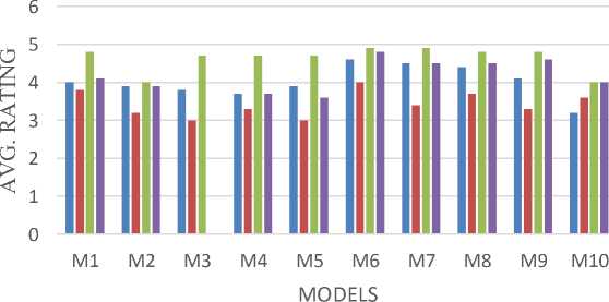
The bar graph in the figure 5 presents the subjective performance analysis of various models mentioned in Table 8. For the visualization, average ratings received from feedback for the generated description by each model is considered. The subjective evaluation reveals no significant disparities in the ratings. Moreover, it demonstrates that Model M6, specifically self-attention enhanced VGG16-LSTM has produced grammatically and semantically accurate description over other models.

■ AC ■ CO ■ GC ■ SC

Fig. 5. Subjective Performance analysis.

The Pearson correlation coefficient analysis was performed between the BLEU scores and the average subjective evaluation scores (Accuracy, Completeness, Grammatical Correctness, and Semantic Correctness) to investigate the agreement between model evaluation metrics and human perception of description quality. As given in table 10, all BLEU metrics exhibit a strong positive correlation with the subjective evaluation criteria (correlation coefficient (r) > 0.75, p < 0.001). Among the objective metrics, BLEU-4 demonstrates the strongest correlation with semantic correctness (r = 0.958), indicating that higher-order n-gram matching more effectively reflects the semantic quality perceived by human evaluators. These findings confirm that improvements in the objective evaluation metrics are consistent with the enhanced description quality observed in the subjective assessment.

Table 10. Pearson Correlation Analysis between Objective Evaluation Metrics and Subjective Human Evaluation.

Objective Metric	Accuracy (r, p-value)	Completeness (r, p-value)	Grammatical Correctness (r, p-value)	Semantic Correctness (r, p-value)
BLEU-1	0.831 (<0.001)	0.804 (<0.001)	0.756 (0.002)	0.852 (<0.001)
BLEU-2	0.874 (<0.001)	0.856 (<0.001)	0.811 (<0.001)	0.891 (<0.001)
BLEU-3	0.912 (<0.001)	0.894 (<0.001)	0.853 (<0.001)	0.926 (<0.001)
BLEU-4	0.946 (<0.001)	0.927 (<0.001)	0.884 (<0.001)	0.958 (<0.001)

5. Conclusion

This study presented a soft attention-enhanced CNN–LSTM framework for semantic description generation from remote sensing imagery. Experimental evaluation on the UCM, RSICD, and Sydney Caption datasets demonstrated that the VGG16–LSTM with soft attention achieved the most competitive performance at a learning rate of 0.0001, where it consistently outperformed the corresponding non-attention variants in terms of BLEU scores. These results indicate that the attention mechanism generates more contextually relevant and semantically coherent description across datasets with varying scene complexity. Despite these encouraging results, the proposed framework has several limitations. The VGG16 encoder produces a fixed-length global feature representation, which may not adequately preserve fine-grained spatial information in scenes containing multiple overlapping or densely distributed objects. In addition, although the attention mechanism improves description quality, the CNN–LSTM architecture incurs increased computational cost due to sequential LSTM decoding and attention computation, making inference slower than fully parallel transformerbased models. The framework also relies on supervised description datasets, limiting its generalization to unseen scene categories.

Future work will focus on using a Vision Transformer (ViT) to capture richer global contextual representations while preserving long-range spatial dependencies. Furthermore, for better understanding of the object relationships graph neural networks (GNNs) will be incorporated. Adaptive multi-scale feature extraction and cross-modal attention mechanisms will also be investigated to improve description quality for complex remote sensing scenes. Furthermore, the model evaluation needs to expand to include more heterogeneous and globally representative datasets like NWPU-RESISC45, to further assess its robustness and generalization capability.

All the Declarations and StatementsAuthor Contributions Statement

Dipti Pawade – Conceptualization, Methodology, and Supervision: Proposed research ideas, Constructed the overall framework, supervised project execution, drafted and revised the manuscript.

Sonali Patil – Writing – Review and Editing, and Project Management: Reviewed and edited the manuscript, ensured clarity and coherence, and helped coordinate project milestones and deadlines.

Riddhi Arya – Model Training, Validation, and Performance Evaluation: Led the model training process, validated results using standard metrics, and benchmarked performance against existing methods.

Hetvi Shah – Model Training, Formal Analysis, Visualization, and Statistical Analysis: Performed in-depth analysis of experimental results, and ensured the statistical robustness of the evaluation.

Diya Bakhai – Data Curation and Software Implementation: Handled data acquisition, dataset preprocessing, and implementing the research model, Writing – Drafted the initial manuscript.

Ankit Jha – Writing – Contributed to the literature survey, and documented the technical background of the study.

All authors have read and agreed to the published version of the manuscript.

Conflict of Interest Statement

The authors declare no conflicts of interest.

Funding Declaration

This research was not supported by any grant or funding.

Data Availability Statement

This study analyzed publicly available datasets. The datasets can be found here: ,

Accessed on October 2024.

Ethical Declarations

The consent has been taken from the people who participated in the subjective evaluation of the generated caption.

Acknowledgments

The authors would like to acknowledge the K J Somaiya School of Engineering, Somaiya Vidyavihar University, Mumbai, India, for providing the computing facilities.

Declaration of Generative AI in Scholarly Writing

AI tool is used to check the grammar and to improve the writing clarity of this paper. They reviewed and edited the AI-assisted content and take full responsibility for the final publication.

Abbreviation

The following abbreviations are used in this manuscript:

LSTM - Long Short-Term Memory

CNN - Convolutional Neural Network

BLEU - Bilingual Evaluation Understudy

RSCID - Remote Sensing Image Captioning Dataset

UCM - UC Merced