Stationary solutions for the Cahn - Hilliard equation coupled with Neumann boundary conditions

We study the steady state solutions for the Cahn - Hilliard equation (see e.g. [2,4,7,8])

u t = ( —au + yu ³ — U xx ) xx , 0 < x < l, t >  0 ,

coupled with the Neumann boundary conditions ux

= u _xxx

= 0 ,

x = 0 , l,

where a and y ^are some physical parameters. The authors of [2] have considered a structure of stationary solutions of problem (1) - (2) as a function of length l and mass m = f l u ( s ) ds. They have counted the total number of monotone solutions, depending on the parameter values of the problem. In [2] phase portraits of the problem have been constructed which describe the monotone solutions for a special stored-energy function f ( u ) + у( u‘ )². wlrere e is a, small parameter. In this case, the function f‘ ( u ) has one negative minimum, one positive maximum, and f ( ±ro ) = ±ro.

In this paper, we study the following problem u" = -au + yu 3 — a, u‘ (0) = u‘ (l) = 0,

where a reflects influence of the average mass on qualitative behaviour of solutions: a is the main parameter of the problem because it is related to an interaction energy of the phase decomposition in a binary alloy; 7 is a parameter corresponding to thermodynamically stability of the system. In particular, a = eBT (1 — T), where Tc is the critical temperature of the phase transition for order-disorder in a disordered binary alloy, which can be measured during the cooling process of the alloy; Eint is the interaction energy between atoms of sorts A and B in the binary alloy. The energy functional corresponding to problem (3) can be written in the form

l

E ⁽ u ⁽ t )) = I Q( u ) 2 + f ⁽ u )^ dx,

E (u (t )) = E (u (0)) ,

where the free energy f (u) is f (u) = 7 u4 - °u2 - au + C.

Note that, in the case a >  0 , be reduced to

7> 0.by the re-scaling u = -   u(^Ox), problem (3) can u ‘‘ = —u + u3 — a,   u ‘ (0) = u ‘(L) = 0,

where L = y OZ and a = a V Y ¹ This case was studied in [2,7]. To the best of authors’ knowledge all other cases were not considered in a literature. Therefore, in this article we investigate the existence of nontrivial solutions of problem (3) for all possible values of these parameters. In particular, we study an interesting case when 7 <  0. It should be mentioned that the case 7 <  0 , a <  0 and |a| < a 0 := 4 JY^ leads to a non-uniqueness result (i.e. there exist two solutions with the same initial energy), depending on initial energy, but the solution of the problem is unique when |a| ^ a 0. Also we describe all possible dynamical scenarios for the parameter values.

Moreover, our results can be applied to the Izing model. For example, the Izing model free energy in the vicinity of the phase transition may be written as the following (see, e.g. [6])

f ( u ) = a + ru ² + su ⁴ + O ( u 6) .

In order for the system to be thermodynamically stable, the parameter on the highest even power of the order parameter must be positive. In this case, we show that s >  0, hence the free energy is bounded. However, for the Neumann boundary value problem we can consider the case when the "open" system is thermodynamically unstable that corresponds to s <  0. For example, in the case s <  0, r >  0 and a G [0 , 2), a solution is not unique. On the phase plane uOu’, this phenomenon is illustrated by two loops with identical lengths of periods which are both symmetric with respect to the axis Ou. Thus, there are two smooth nontrivial solutions.

1.    The Steady State Solutions for the Cahn - Hilliard Equation

In this section, we find the existence interval, L for a monotone solution by considering all possible values of the physical parameters. We proceed by examining all qualitatively different nine cases. Note that since all systems at hands are conservative they cannot have any attracting fixed points. Therefore their phase portraits can have only saddles and/or centers.

I.В. Krasnyuk, R.M. Taranets, M. Chugunova

-ЧП.

XXX 2-Ul

11 tt

XXXI

fl

ft tt

Xll^ ttt V tttt

TT ft tt

0- '

-1

2 xxx

4 4 4/

-2

tf T

ttt

I -■

У

/Mt

At

ttt

.ttt

tt tt

o-'

-1

Xittxxxvvxv XXXXXXXXXXX 44444444444

\Wt

XXft '

JMt ■ 44A4

Wit fttt ttt

ttt

ttt ttt

44 44

3 4 44

-2

-1

чг*,«'^«'*~\

tt tt tt tt

и

Fig 1. Phase diagram for the case a >  0 , y >  0 ^with a = 0 , 1 on the left and a = 1 on the right

• 1.1.    Case a >  0 , y >  0

  In this case, by the re-scaling u =

  
  

au(Vax), problem (3) can be reduced to u ‘‘ = —u + u3 — a,  u ‘ (0) = u ‘ (L) = 0,

where L = д/ a/ and d = aVY* Integrating (6), we find that

( u ‘ )²     u ⁴ u ²                               1

• —---4 + — + au = p -. ( u‘ )² = ^( u ⁴ — 2 u ² — 4 au + 4 p ) .

Note that the equation u ³ — u — a = 0 has

• •    three real roots

2   z,2kn ф = jarcc0^3/^);

uk = —p cos( ф + -—) , k = 0 , 1 , 2 , з 3

provided that a ² <  27 (two minimums and one maximum). Thus, we have two nontrivial u ˆ ⁴         u ˆ ²                                  u ˆ ⁴         u ˆ ²

solutions if —max + ^m₂ + au _max < p <  —min + -^ + au min and the lengths of intervals, where the corresponding solution has only one zero, are

L 0 , 1 =

V2

u 2

/

u 1

dt

/t ⁴ — 2 t ² — 4 d t + 4 p ’

u 4

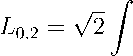
u 3

dt

/t ⁴ — 2 t ² — 4 a t + 4 p

where u k are four real roots of the equation t ⁴ — 2 1 ² — 4 at + 4 p = 0 such that u 1 < u 2 <  u ˆ ⁴         u ˆ ²

u3 < u4. We have only one nontrivial solution if p < —max + -л2ах + arzmax with the length of interval, where the solution has only one zero, given by u2

L 0 , 3 = V ² j

dt

л/ 1 ⁴ — 2 1 ² — 4 d t + 4 p¹

u 1

ttttt

> х х 4 4 4 4

।

ttttt ttttt

u' O-.

ttttt tf ft t ttttt

444 4444 XV 4 4 4 4 4

2 tttt tttt

1 tttt

—

ttttt

-3

-2

t| tl

-1

о

и

V 4

/

4 4444

J 44444 . 44444 ■ 44444 144444

V/44444

«■

0-.

-1

ttt ttt

ttt

tttt tttt tttt

2 tttt

ttttt

-3

-2

-1

О

и

A V VI

/41 V4S /#4

i

4 4444 44444

Fig 2. Phase diagram for the case a > 0, y < 0 with a = 0,1 on the left and a = 1 on the right where uk are taco real roots of the equation t4 — 2t2 — 4dt + 4p = 0 such that u 1 < u2:

• •    one real root

a    /12    1" \1 /³    a    012

-

1 )1 /³

27/

u min 2' W — 27) + C V T uˆ4

provided that a²> 27 (one minimum). Tims, we 1 iave a nontrivial solution it p < —m + uˆ²

₂ + aumin with the length of interval, where the solution has only one zero, given by

L 0 = /

u2

dt

/t4 — 2t2 — 4 a t + 4p, u1

where uk are two real roots of the equation t⁴— 2t²— 4dt + 4p = 0 such that u 1 < u2:

• •    two real roots                    _{a                a}

umin = ²⁽ |)1 /³, ^ufl = ^{— (}|)1 /³

provided that a²= 27 (one minimum). Tims, we 1 iave a nontrivial solution if p <

umin + aumin = 2(-2)²/³with the length of interval, where the solution has only one given by

⁴ umin

4 ⁺

zero,

u2

L0 = /2 /        dt      = ,

J V t4 — 2t2 — 4 at + 4p u1

where uk are the two real roots of the equation t⁴— 2t² + 4at — 4p = 0 such that u 1 < u₂.

Thus, if 0 < L < L0 then the corresponding solution of the problem has no zeros located on the interval (0, L). If kL₀< L < (k + 1)L₀, where k = 1, 2,..., then the solution lias exactly k zeros located ,L).

• 1.2.    Case a > 0, y< 0

In this case, by the re-scaling u = . —au(/ax), problem (3) can be reduced to u ‘‘ = —u — u3 — a,   u ‘ (0) = u ‘ (L) = 0,

(П)

I.В. Krasnyuk, R.M. Taranets, M. Chugunova where L = y^Z and d = aV-a• Integrating (11), we obtain

(Ui, ‘ )2 Ut⁴ u²                               „     1

—--+ — + — + du = p -^ (u‘)² = ^(—u⁴ — 2u²- 4du + 4p).

Note that the equation u³ + u + d = 0 has only one real root

„       ( d     П2    Гx¹/³      d     /d²    1" x¹/³

umax = W 2+VZ + 27)  + I" 2 -V Т + 27/ for any d G R1 (one maximum). Thus, we have a nontrivial solution if p > umax + umax + dUmax with the length of interval, where the solution has only one zero, given by u2

L⁰ = V.

dt

/—t4 — 2t2 — 4 d t + 4 p p u1

where uk are two real roots of the equation t⁴ + 2t² + 4dt — 4p = 0 such that u 1 < u₂. For example, if d = 0 arid p > 0 then we have

(u' )² + (u² + 1)² = ₁,

where A² = 4p+l, В⁴ = 4p + 1, and from (13) it follows that

B²-1                                1

В²    Г         dt _ ~ Г dt

A J   ^/в⁴— (t² +1)2 = J vci — 1²)(i+к2Я’

-^√B²-1                         ^-1

where

A=

B²

A^B² + 1 ’

k²

B²— 1

B² + 1

G (0, 1).

Let t = sin ф in integral (14). Then

L0 = 2A

π/2

dφ

/1 + k² sin²ф

L₀G (2.622A,nA).

• 1.3.    Case a < 0, y > 0

In this case, by the re-scaling u =   —au(V—ax), problem (3) can be reduced to u ‘‘ = u + u3 — d, u ‘ (0) = u ‘(L) = 0,                       (17)

where L = V—a Z and d = — a \/—a • Integrating (17), we obtain

(u, ‘)²     ? 1⁴     ? 1²                                      1

—2---4 — — + dU = p ^^ (u‘)² = ^(u⁴ + 2u²— 4du + 4p).

Note that the equation u³ + u — d = 0 has only one real root

„       / d     /d²    1" x¹/³    d     d²    Fx¹/³

^u min ⁼(2 ⁺ VZ⁺27) ⁺G ^— VT ⁺ 27t

444 444

trt

3 1444 4

2 111

I

444 -444

ttt ttt

u' 0-'

44 V 144

ft tt

trt

ttttt ttttt

u'

-I

44/

4 4yV

ttttt

Vt 1111

2 4 4 4

-3

4 4 4#

44 4 /

-3

-2

-1

44444V

2-4444 4 V 444444 444444

i t/t t t ^rr tit 11

i

4444444V 4444444V 44444444

ttt

0-'

Ht ttt ttt

ttt ttt

-I

tttttttw^ 4444444/

ttt

ttt

ttt ttt ttt ttt

Fig 3. Phase diagram for the case a < 0, y

the right

Al t t ; z^-*-*->-<-f->->->s\ 4 4 4 4 1ttt7 >-»->-♦->-►-►-»->'> у V 4 4 4 tttt/ л-*-*-*-*-*-*-*-*ч У V 4 4 4

ttttf

i -

0-.

tttt tttt tttt] tttt tttt

2 444 44/y

ttt

44 4 4

-3

-2

-1

I

-1

tttt1» ttttt

-3

-2

I

и

Fig 4. Phase diagram for the case a < 0, y

tt tt

> 0 with a = 0,1 on the left and

CT = 1 on

u'

ttt Г ttt»

2 tt t

i -

0-.

-1

ttt ttt ttfl tt tt tt tt

tt

ttt ttf

ttt^a tttt

-3

Zy

-2

Л4444 > 4444

f 44 t44

4 4

4 4 Z4

Qitttt t/t tttt

-1

о

и

i

< 0 with a = 0, 1 on the left

and a = 1 on

the right for any a E R1 (one minimum). Thus, we 1 nwe a nontrivial solution If p > — umin — umn + aumin with the length of interval, where the solution has only one zero, given by

L о =

V2

u2

/

dt

//t⁴ + 21²— 4 a t + 4 p p

where uk are two real roots of the equation t⁴ + 21²— 4at + 4p = 0 such that u 1 < u₂.

• 1.4.    Case a < 0, y< 0

In this case, by the re-scaling u = . -дu(V—ax), problem (3) can be reduced to u ‘‘ = u — u3 — ст,   u ‘ (0) = u ‘ (L) = 0,

I.В. Krasnyuk, R.M. Taranets, M. Chugunova where L = V-a l and d = — ^VY' Integrating (19), we find that

(Ui ‘ )2    u⁴    u²                           „     1

• —--+ —---^ + du = p ^, (u‘)²= ^(—u⁴+ 2u²— 4du + 4p).

Note that the equation —u³+ u — d = 0 has

• • three real roots

uk = —cos(ф + ^2кп), k = 0,1, 2, ф = ¹ arccos(³^^d); V 3   3      ³²

provided that d²< 27 (two maximums and one minimum). Thus, we have two nontrivial solutions if umax — umax + dumax < p < umin — umi¹ + du_min with the lengths of intervals, where the corresponding solution has only one zero, given by

L 0,1 =

u2

/

u1

dt

У—1⁴+ 21²— 4 d 1 + 4 p ’

u4

u3

dt

У—1⁴+ 21²— 4 d 1 + 4p

where uk are four real roots of the equation 14 — 212 + 4d 1 — 4p = 0 such that u 1 < u2 < u3 < u4.

uˆ⁴        uˆ²

We have only one nontrivial solution if p > -^--min + dumin with the length of interval, where the solution has only one zero, given by

L0,3 ⁼

u2

/

u1

dt

У—1⁴+ 21²— 4 d 1 + 4p ’

where uk are two real roots of the equation 1⁴— 21²+ 4d 1 — 4p = 0 such that u 1 < u₂: • one real root

( d     /d² Г \¹/³d /d²"

1 у /³

27/

umax

= Г 2 ⁺ VT — 27) ⁺ 1— 2 — V "4"

provided that d²> 27 (one maximum). Thus, лае have a, nontrivial solution If p > umax — uˆ²

-J2ax + dumax with the length of interval, where the solution has only one zero, given by u2

L0 = v2 / u1

dt

У—14 + 212 — 4 d 1 + 4p ’ where uk are two real roots of the equation 14 — 212 + 4d 1 — 4p = 0 such that u 1 < u2: • two real roots umax

—2(d)¹/³, df. = (ф¹/³

provided that d²= 27 (one maximum). Thus, лае have a, nontrivial solution If p > umax —

² umax

2  + и umax given by

—2()²/³with the length of interval, where the solution has only one zero,

u2

L0 = V2 у u1

dt

У—1⁴+ 21²— 4 d 1 + 4p¹

14V

2 111 ЦК liny 11141 14444» 444441 44444

V

T o-'

—

ini

Ч

2 44 4 tj 444#

-3

-3

-2

-1

о

и

ttt fit tft ttt

tttt

tifttttt tilt tttt

tttt tttt tttt to ttt л ttt

и

■'

ttttf

tttti

1 т T T ttt

О Ш

-1

ttt ttt

tttt tttt

.мин

к

ШЛ QtT nt t It I 4t\ th v

>4U

ttttt

-3

-2

-1

ll

/«4

4 4 44

i

Fig 5. Phase diagram for the case a = 0, y > 0 with a = 0,1 on the left and for the case a = 0, y < 0 with a = 0, 1 on the right where uk are taco real roots of the equation t4

^^^^^^^^^r

21² + 4at — 4p = 0 such that u 1

< u2-

For example,

if a = 0 arid p > 0 then we have

where A¹²

4p+1 2

B⁴ = 4p + 1.

L₀

B²

A

A^{2 +}

and from

B²+1

^{∫  √}B4

^√B²+1

dt

(u 2 — 1)2_{= 1} B⁴        ’

(24) it follows that

-

1)2

¹f

-1

dt

V(1 - 1²)(1 + k²12) ’

where

A=

B²

aVb²— 1 ’

k²

B² + 1

B²

-

> 1.

Let t = sin ф in integral (25). Then

π/2

L о = 2 A

dφ

V1 + k² sin²ф

< π A.

• 1.5.    Case a = 0, y = 0

If a = 0, y > 0, by the re-scaling u = u(/x), then problem (3) can be reduced to the one u ‘‘ = u3 — а, u ‘ (0) = u ‘(L) = 0,                           (28)

where L = /^l and a = — T Integrating (28), we find that

(u.‘)²     u*                                      1

—2---4 + au = p ^^ (u )² = ^(u⁴— 4au + 4p).

I.В. Krasnyuk, R.M. Taranets, M. Chugunova

Thus, problem (28) has a nontrivial solution provided that p > 4d^4/3, i. e. p > 4(^)⁴/3.

The length of interval, where the solution has only one zero, is

L0 - V2

u2

dt

V t⁴- 4 dt + 4p¹ u1

where uk are two real roots of the equation t⁴— 4dt + 4p — 0.

If a — 0, y< 0, by the re-scaling u — d(V—Yx), then problem (3) can be reduced to

u ‘‘ — —u³— d,  u ‘ (0) — u ‘ (L) — 0,

where L — V—Y l^and d — T Integrating (30), we find that

(u ‘ )²    u⁴                                 1

—--+ — + du — p < > (u )² — ^(—u⁴— 4du + 4p).

Thus, problem (30) has a nontrivial solution provided that p > — 4d⁴/3, i. e. p > — 4(^)⁴/3.

The length of interval, where the solution has only one zero, is

L 0^—V2

u2

dt

V—t⁴— 4 dt + 4 p ’ u1

where uk are two real roots of the equation t⁴ + 4dt — 4p — 0. For example. if d — 0 and

p > 0 then we have the сште

(u' )²    u⁴

A^{2 +}B⁴    ’

where A² — 2p, B⁴ — 4p. Obviously, the length of interval, where the solution has only one zero, is

B1

B²dt 2B dt B _ Д L B 2,622

^L 0 ^—A J VBA—T4^—A J VT—T* " 2A^B( 4 ’ 2) ~²’⁶²²A^—"YT •    ¹³³¹

-B                   0

where B(a^b) :— J xa^- 1(1 — x)^b-1dx is the loeta, function.

• 1.6.    Case y — 0• a G R¹

If a — 0• Y — 0 then problem (3) can be reduced to

■V^м — —di   u‘ (0) — u‘ (l) — 0.

This problem has the following solution u (x) — C V C G R1 aiid d — 0 • and it has no solutions if d — 0.

I

-ZZZA tttl tttfr

л V X У V

3 -

2 -

о-.

-I

11 te уу у\ у у у v у УХУ

^тг т t Л

УХ V

-з

-2

-1

О и

^у аЛу у IU

V * 4 4.

у у у у у i у у бууу

i*у г Дг/г 44 4 4 4ii4

1           2           3

1 -

X X X X XX УУУХХУ

ти

У У У У У У У »>'«-♦ Z/ rtttttt

0-

-I -

у 4 4 ill 44/4 444444 4»/ 444 44 /*

ХУУУУ

-2 -

-з -

-з

-2

-1

I

УУУ

Fig 6. Phase diagram for the case a > 0, y = 0 with a = 0,1 on the left and for the case a < 0, y = 0 with a = 0, 1 on the right

If a > 0, y = 0, by the re-scaling u = u(/ax), problem (3) can be reduced to u ‘‘ = —u — a,  u ‘ (0) = u ‘ (L) = 0,

where L = /al and a = a- This problem has the following solution

πk

u(x) = C cos(/ax) — a, l = —=, k E Z +, C E R¹. α

If a < 0, y = 0, by the re-scaling u = u(/—ax), problem (3) can be reduced to u ‘‘ = u — а,   u ‘ (0) = u ‘(L) = 0,                           (36)

where L = /—a l and a = — Д This problem has the following solution u (x) = a.

For convenience, we summarize our existence results in the form of Table.

• 1.7.    Example

As shown in [3], the possible dimensionless function f (u,T) at hxed T can be written

Tn    232   T — T0, ^332^ C_T1 ( T )

f(u,T) = 4T0(1 — u ) + a to (u + 1) + foTln I to , where T0 is a, critical tnmperature. c is the heat capacity, a = 4^0 is dimensionless. I is the latent heat, f0 is a parameter with dimensions of energy density. Comparing (37) with our f (u). we hud that

T T — 2 a (T — T0)      2 a (T0 — T)

• ¹    = To ’“ = To,      ’ ^a = TO ’

C = cT ln (^T) + T^{+ 4}“(T — T0>.

^f0       ^T0 /         ^{4 T}0

I.В. Krasnyuk, R.M. Taranets, M. Chugunova

Table

Conditions on the problem’s parameters for existence and non-existence of nontrivial solutions

α	σ	γ	p	L0
> 0	2    4α3 σ < 27γ	> 0	p C [pmin, pmax )	Yes (2 sol’s)
> 0	2    4α3 σ < 27γ	> 0	p < pmin	Yes
> 0	2    4α3 σ < 27γ	> 0	p ≥ pmax	No
> 0	2    4α3 σ ≥ 27γ	> 0	p < pmin	Yes
> 0	2    4α3 σ ≥27γ	> 0	p ≥ pmin	No
> 0	R1	< 0	p > pmin	Yes
> 0	R1	< 0	p ≤ pmin	No
> 0	R1	= 0	R1	Yes (family sol’s)
< 0	R1	> 0	p > pmin	Yes
< 0	R1	> 0	p ≤ pmin	No
< 0	2    4α3 σ < 27γ	< 0	p C (pmin, pmax]	Yes (2 sol’s)
< 0	2    4α3 σ < 27γ	< 0	p > pmax	Yes
< 0	2    4α3 σ < 27γ	< 0	p ≤ pmin	No
< 0	2    4α3 σ ≥27γ	< 0	p > pmin	Yes
< 0	2    4α3 σ ≥27γ	< 0	p ≤ pmin	No
< 0	R1	= 0	R1	No
= 0	R1	> 0	p> 3 (3 )*/3	Yes
= 0	R1	> 0	p < 3 (' )*/3	No
= 0	R1	< 0	p> -3(3)4/3	Yes
= 0	R1	< 0	p < 3 (3 )*/3	No
= 0	R1	= 0	R1	No

For example, if 0 < T < T0 then a > 0, y > 0, ^and ст > 0. In this case, according to the paragraph 2.1, problem (3) has nontrivial solutions. On the other hand, if T > T0 and a ^< 2(T^T-T0) then a > 0, y > 0, ст < 0 and we again have the existence of nontrivial solutions.

2 . The Steady States for General Free Energy

In the previous section, we have studied the case when the free energy contains the linear term but it has no cubic term. Note that the presence of a linear term breaks down the symmetry of the free energy. Next, we will examine how the length of the existence interval can be effected by the cubic term. It is possible to introduce asymmetry in a phase diagram by adding odd powers to the free energy expansion so that f (u, T ) = a 0(T) + a 1(T ) u + a 2(T )2 + a 3(T )"3 + a 4(T )^ + O (u 5) •      (dS)

Note that the special case a 1(T) = a3(T) = 0 was introduced in [6, p. 19, (2.41)]. The authors assumed that a₄(T) > 0 and a₂(T) < 0. Then f(-,T) has maximum at u = 0 and minimum at -± = ±\j-a4• By definition, it is easy to verify that f (0, T) = a₀(T) > 0 and f (-±,T) < 0 as a2 > 4a0a4 > 0. It means that there is a point -0 G (0, — OJ) such that f (±-0, T) = 0. Thus, we can calculate the minimal length as

L₀

-u0

dt

Vt—u 0⁾⁽t²-ul)

V a 4 -² /

-1

dt

^V(i — 12)(i —"Pty’

where

^u0 = A----a/a2 -⁴a0 a4, ^u 1 = A /---1--J^a2 ^{— 4}a0a4

a4   a4                           a4   a4

k²

-0 G (0,1). (40) u₁

Substituting the new variable t = sin ф into (39), we have

L = ₂ПЕ [^n/2 a4u²_{1 0}

dφ

V1 — k² sin²ф

Next, consider the ecpiation

1       „

₂(-' )² = R (-)

then

u2

L - =^j u1

dz

VW) ’

vdiere -i are real roots of R(-) = 0 such that - 1 < -2. Here

R (z) = az⁴ + bz³ + cz² + dz + e = a (z² + pz + q)(z² + p z + q')         (43)

where a, b, c, d, e, p, q, p, q' G R, a = 0, i. e.

be + (ad — bc) q .

p =-------1^-’ p =

a(2e — cq)

be - adq _′e

a(2e — cq) ^,

q = —’ q = aq

1 c i c²— 4 ae A    ₂    .

2 ^ ±V a^) ’ c > ⁴ae'

Note that (43) has four real roots

^-1,2 = 2 (—p ± Vp^{2 — 4}q)

’ -з,4 = 2 (^—p‘ ± V⁽p^{)2 — 4}q‘)

provided that p2 — 4q > 0 and (p‘)2 — 4q > 0.

Assume that p = p'. By change of variables

^t±V     ^ ^{— v}

^zt + 1 ’ ^z    (t +1)^{2 dt}

I.В. Krasnyuk, R.M. Taranets, M. Chugunova in (42),

we deduce that

L 0 —

µu₂ +ν ^u2                    ^u2⁺¹

— A /

2 J Rr)P J u1                   µu1 +ν u1 +1

dt

V(1 + k 11²)(1 + k2t2) ¹

where

A —

µ

-ν

²   a (v² + pv + q)(v² + p'v + q')

Here,

µ

k_—ц² + pц + q k_—ц² + p' ц + q' ¹   v² + pv + q ’²v² + p' v + q'

and v can be found from equations

p (ц + v) + 2( q + цv) — 0, p (ц + v) + 2(q' + цv) — 0,

hence v—

_q′ _-

p-

q± p′

-

pq′ p′

-

-

p′q

, ^{ц p}

_q′ _-

p-

q∓ p′

-

pq′ p′

- p^′q

.

-p

If (43) has four real roots then ki < 0. By change of variables t — (—k 1) ¹/² sin ф in (45), we deduce that

φ2

L о = Ai φ1

dφ

V1 — k3 sin²ф

where

A — -A

-

=, kз — 27 > 0, фi — arcsin ( ^  ¹⁽^ui^+v)) .

k i k 1                   V     Ui + 1     /

In particular, if (43) has only two real roots then k 1 < 0 and k₂> 0 оr k 1 > 0 and k₂< 0. Moreover, if a > 0 then the problem has no solutions therefore we have to consider the case a < 0 only. Ass nine that k 1 < 0. Then we olot ain (48) with k 3 < 0.

In the case p — p'. by change of variables z — t — p in (42). we deduce that where

u2

y/2 Г dz

^{0  2}J ^RT)

u1

p u2 -₂

—A

u1

p

dt

^, у a(1 — k11²)(1 —^Z21²)

_z              2y/2

V( p^{2 — 4}q⁾⁽p²

-

Z

^=^, k^ — 4 q')

_p2 _-

/X

>⁰, ^k 2 ^—

4q

—--— > 0.

p²— 4q^'

By change of variables t — (^k1) ¹/² sin ф

in (49), we find that

φ2

L о = M

φˆ1

dφ

\ja (1 — k₃ sin²ф)

where

Z k3 = У > 0, фi = arcsin f Vki(ui — p/2) ) . k1

Next, we consider the special cases p² = 4q оr (p')² = 4q‘. For example, if (p‘)² = 4q‘ then

-p - Vp²-⁴q       -p + Vp²-⁴q ( .p')²

R^(u) =     --2-----) (^u--2-----) Г ⁺2j •

If a < 0 then two cases are possible:

⁽i)

-

p′

2 E

—p — Vp²— 4 q

I ²        ’

—p +

Vp²-⁴q

²        )’

⁽ii)

(

-p

-

Уp²— 4 q

—p + Уp²— 4 q 2

)

In the first case (i), we find that L0 = to. In the second case (ii), we have (48). On the other hand, if a > 0 then the problem has no solution in the case (i) but for the case (ii) we have L0 = to.

In particular, if p² = 4q arid (p‘)² = 4q then

R (u) = a

(u + p)² (u₊y.

Obviously, if a < 0 then the problem has no nontrivial solutions but if a > 0 then L0 = to.