Structural Methods of Estimation Lyapunov Ex-ponents Linear Dynamic System

Published Online September 2015 in MECS

Methods of parametric identification are quite a settled theory. The problem of structural identification (SI) dynamic systems has not obtained the definitive solution. Different factors influence a solution of problem SI. Some of them in [1] are considered. The essential factors:

• i)    difficulty of formalization of a problem in mathematical terms;

• ii)    lack of strict dependences between structure parameters (SP) and reflecting processes in a system the experimental information;

• iii)    presence of "impeding" interdependencies between variables which about SP a complicate decision-making process.

Complexities of a problem structural identification are noted in [2]. Therefore, problems of structural identification more often at some level of the a priori information [3] solve. Such approach the class of mathematical operators which describe a behaviour of system on available informational set narrows down. Direct methods of identification structural parameters and performances even in such statement of the problem are not applicable. Estimations SP indirectly on the basis of an application of the different criteria characterizing quality of obtained solutions, define.

To research in the given direction of the theory of identification systems symposiums and conferences [4, 5] are devoted. The majority of offered approaches to application of various methods approximation model system on the given set of polynomials or functions are based. As a rule, parametric approximation is applied to the set class of models applied. The natural path of a solution of an existing condition is introduction of different heuristic procedures structural identification which considers features of a studied problem. They are grounded on an application of neural networks, intellectual and genetic technologies [6-13]. Application of these technologies is grounded on learning of their elements by means of search models-applicants and obtaining of total adequate model. Such approach does not bring in anything new to problem SI. It is based on a parameterization paradigm. Structure choice is an approximation co-product.

So, the analysis of works will show that in systems of structural identification the parametric approach to the set class of polynomials or functions is dominating.

In [14] the approach to a problem of the structural identification, based on the analysis special (virtual) SK -structures, is offered. They characterize a condition of a nonlinear part research system. The analysis of properties system is fulfilled in special structural space. Development of the given approach is given in [15, 16]. Further we will state application of the given approach to a problem of an estimation LE.

Now for the analysis of qualitative behaviour dynamic systems widely use Lyapunov exponent. They are applied to an estimation of behaviour of trajectories of different plants in the physicist [17], medicine [18], economy [19] and astronomy [20]. Lyapunov exponents estimate on the basis of the analysis time series. The a priori information on system structure is supposed known. In [21] survey of an evaluation of the largest LE for different classes of systems is given. In [22] the algorithm of estimation LE of unknown dynamic system is offered. The algorithm gives estimations for all LE. It on application of networks with multivariable prediction is based. Monotonic sigmoid functions as a base of a network are used. The problem solution as selection of parameters of the functions approximating a time series by square-law criterion is given. From the analysis of works we obtain that in the majority of publications application LE is restricted by research of qualitative behaviour system. Other problems of the theory of identification will not be researched. Therefore, it is necessary to embroider area of the analysis performances LE for a solution of a wider spectrum of problems identification. To them we and a problem of structural identification will refer. The analysis of publications will show that from such positions of research were not fulfilled.

We a method of solution a problem structural identification linear dynamic systems on the basis of the analysis Lyapunov exponents in the conditions of a priori uncertainty offer. Solution of the problem we on the basis of the analysis the experimental information on system work search. For an evaluation of spectrum LE, the approach offered in [15, 23], is used. The method of estimation the general solution system on the basis of application static model is developed. Definition of Lyapunov exponent (LE) on the analysis of a coefficient structural properties system is based. On the basis of a coefficient of structural properties the special structures reflecting change LE are introduced. The criterion of estimation an order system on the basis of the analysis behaviour these structures are offered. Two approaches to an estimation of the largest LE and the least indexes of Perron are offered. The first approach on identification of a change a coefficient of structural properties with the help secant method is founded. The second approach is the structurally-frequency method grounded on definition of estimations LE by means of the analysis of local minima of structures offered in work. The frequency method which is a modification of a method a bar graph in the statistical theory is applied to a validation of the obtained estimations. We offer the algorithm of an estimation of Lyapunov exponents in the conditions of uncertainty. It allows defining the type of eigenvalues and an order of a dynamic system.

• II.    Problem Statement

Consider linear dynamic system

X = AX + BU ,                  (1)

Y = CX + DU, where X g Rm is a state vector, U g Rk, Y g Rn are an input and a system output, B g Rmxk , C g Rnxm , D g Rnxk.

For system (1) the experimental information is known

I o = { Y ( t ), U ( t ), t g J = [ t 0 , t , ] }              (2)

Solution of system (1) note in a form

X (t ) = X ( t 0 , U , t )                    (3)

where X is an operator uniquely defined by matrixes A , B .

On the basis of (2) from (3) we obtain a solution of the system (1) at X _o = X ( t ₀)

X(t ) = X g (t ) + X q ( t )                 (4)

where X_q ( t ) is a particular solution (1) with U g I_o , X_g ( t ) is a general solution (1) with U(t ) = 0 with an unknown vector X_o g I_o .

We designate the general solution (1) with X 0 = X o ( Y o ) g I o as X g ( X 0 , t ).

Problem:     to     find     solution     estimations

X_g ( t ) = X_g ( X_q , X _o, t ) on set I_o and to make a solution of a spectrum of eigenvalues and an order of the system (1).

• III.    Estimation X ( t )

For estimation ХПЛ generate set { X_g ( t ) } . Fulfil for this purpose operation { X ( t ) } \ { X_q ( t ) } and apply the approach, offered in [14].

We will state a problem method of solution on an example of a system (1) second order with one input and an output. Designate y = Y ; u = U . Let D_y ( ш ), D_u ( ш ) are frequency spectra of signals u , y , | y(t ) | < ^ , | u ( t ) | < ^ . Let D_y ( ш ) = D_u ( ш ), that is the system (1) is linear and stationary. Real parts of roots ^ a performance equation of a system (1) at the made assumptions are negative: Re ^ <  0, i = 1,2.

Present I as

I o = I q ( J q )ui g ( J _g )

where J U J = J c R ; I q , I g are sets which contain the information about X and X .

On the set find an estimation of a particular solution system (1). As x_x = y g R , for deriving components x₂ = x of a vector X g R ² use operation differentiation of a variable y . Let x ₂ = y .

Statement 1 [14]. To identification X ( t ) on set I ^q apply model

J X q ( t ) = A q W ( t )    V t G J q            (5)

where A e R ^2x2 is a matrix of parameters of model, W = [ u u 'f .

The proof of statement 1 is grounded the account of phase shift between u '( t ) and u ( t ). Therefore we apply a least-squares method to deriving of a matrix A ^ˆ and we ensure compensating for time delay in a system (1).

Properties of the model (5) depend on choice of interval J c J . The model is applicable and for a case m >  2 .

We on the basis of the model (5) on set I ^g define an estimation of a particular solution X ^ˆ ( t ) of a system. Further we find an estimation of a general solution

Xg (t) = X(t) - XTq (t) Vt e Jg where XTg(t) =[ yg (t) yg(t)] .

The offered approach is easy for generalizing from a multidimensional case.

Further, we consider a system (1) with one input u and an output y .

• IV.    About Identifiability of Model (5)

Model (5) is applicable only to the certain limitations superimposed on an input of system u ( t ). The input should be extreme nondegenerate restricted. This known demand to signals in identification problems. At level of a phase portrait S identifiability of system corresponds to closure S . It is not complicated to prove this demand. So, the structure S should have followed the property of identifiability.

The system (1) is h -identified if the structure S is closed, and the distance h between two opposite points S is not less 8_h ( 5_h >  0 ) for almost all t e J .

• V.    LE. System Coefficient of Structural Properties

We will apply Lyapunov exponents [24] to an estimation of a spectrum eigenvalues dynamic system (1). LE use as a system stability criterion. For a real-valued function h ( t ) LE defines as

x [ h ] = lim ^ln h ⁽ t )                    ⁽⁶⁾

t ^”    t where lim is a limit superior. t ^w

LE x ( i = 1, m ) solution of a stationary system (1) coincides with real parts of eigenvalues ^ of a matrix A .

Let the estimation of the general solution X(t) of the system (1) is known Vt e J' . We suppose that the system is stable. Apply (6) to yˆ (t)

^x [ ^y g 1= “m

ln y ˆ g ( t )

t

where t e J_g is the maximum value t on the interval J g c J .

X [- y g 1 is the largest LLE. If the limits (6) exist, X [ y ^g 1 is an estimation of a maximum eigenvalue of a matrix A . So, x [ T _g ] is an index of degree stability system (1). If m = 2 , for y_g obtain

X

ln y ˆ g

= lim—^!—¹ t ^ t      t

Also use an index ln h(t)

П[ h ] = lim—!1 t >w      t where lim is a bottom limit. It is the Perron bottom index t ^w

Further we show a mode of estimation n [ h ] and its interdependence with a system spectrum.

On the basis of the analysis x [ y_g ] , _X [ "y_g ] and their transformations we algorithms of decision making about type of roots and a system order offer.

The idea of the application of Lyapunov exponents in identification problems is explained in [14, 23]. The offered approach on the analysis of a coefficient of structural properties (CSP) [14] is based. Further, we give development of the given method. Display at first interdependence between CSP and LE.

Introduce for system (1) index

p(y g )=pg = lnlyg (t)  Vt e Jg c Jg where Jg = [t0, t ] define on the basis of (7).

Consider system with an input t and an output p( ^yg). Introduce CSP for an estimation of structural properties this system ks (t, p) = ^iyyg!                 (8)

k (t, p) is the basic variable for a computing of an index x[yg ] on the interval Jg . We consider ks (t, p) as a transfer constant of a system with an input t and an out put p(yg). Further, we for an estimation of characteristic indexes will state a mode of application ks (t, p).

So, we between LE % [ y _g J and a coefficient of structural properties k_s ( t , p ) on informational set I _p = { p ( y_g ( t ) ) , t g J_g } showed interdependence.

Consider set

Ig ( Уg , t ) = { yg (t) , t G Jg } = IXg \ { yg (t) t G Jg } , which contains the data for a variable change yˆ in the interval J .

We suppose that the system (1) is stable. Then Re( Z ) <  0, г = 1, m , where 2. g a (A) is i -th eigenvalue of a matrix state.

Problem: on the basis of the analysis of sets I , I a spectrum ^ ( A ) of eigenvalues a matrix A system (1) and its order estimate.

Problem solution reduces to implementation of following stages.

• 1.    Definition of an order system.

• 2.    Definition of initial estimations for a spectrum of matrix A .

• 3.    Development of an adaptive algorithm for an improvement of the estimations obtained at a stage 2.

Adaptive algorithms are obtained in [14]. Therefore, here they are not considered.

The basic difficulty of application of least-squares procedure is approximation y ˆ ( t ) on the class of functions { е ^л ' , i = 1, n } . e ² i t nonlinearly depend from 2. .

At a stage 2 we consider a type of roots of a dynamic system. Algorithms for decision making on the analysis of the structures reflecting properties LE are grounded. Further, we introduce these structures.

• VI.    Structures for Estimation LE Consider sets

^I k s = { ^ks ( t , P ⁽ y g ⁽ t ) ) ) , t ^{G J}g }

I k S = { k s ( t , ^{p У}g ⁽ t ) ) ) , t ^{G J}g }

Define on I , I^, map Sk  ^ I, x Ik, . The structure s       ss                 ss, p          ss       ss

S of a time history of the indexes depending from LE, reflects. Consider on set I the function describing a change of the first difference k_s ( t , p ( y _g ( t )),

^A k s^(t ) = k s ( t , p ( ^yg ^{( t} + ^{t )} ) ) - k s ( t , p ( ^yg^(t ) ) )

where т >  0.

Generate set 1_дk, = {a k_s ( t , p ( y _g ( t ) ) ) , t g J_g } and consider the structure SK^_k, ^ I^ x I^ , . Except structure SK^_k, consider transformation corresponding to it

LSK ^{a k}V p ^ I ks , p ^x B ⁽ I ^{a k}V p )

where

B ( I a k s, p ।    { - 1; 1} . Elements of binary set

B ( I Ak s, p ) define as

[  1, if Ak' (t) > 0, b (t) =               ,        ’

[-1, if ak; (t) < 0, t g Jg

Remark 1. For some class of systems on the basis of a change S we can choose limit superior boundaries in (7).

Remark 2. We define choice of a range function b ( t ) by convenience of its graphical analysis. Its defined for binary set {0;1} .

• VII.    Estimation of Order System

We give a criterion of an estimation an order system (1) on the basis of the analysis properties of the structure LSK Ak s , _p .

Theorem 1. The system (1) has an order m if function b ( t ) on the interval [ t ₀, t * Jc J_g ( t * <  t ) changes the sign m - 1 of times.

Proof. Consider a case of simple real roots. The system (1) is stable. Let ^S is a structure describing a phase portrait of a system (1) with output y g R by means of function Г : y _g ^ y_g . System eigenvalues are arranged in decreasing order ^ >  ^ > ... >  ^ . The phase trajectory at prevalence of each component e ^{X it} g y_g on some subinterval J_x c J changes an angle of inclination. Such process can happen exactly m - 1 time. As function the p ( y _g ( t ) ) depends from y _g ( t ) each such change transform to a change of properties of structure LSK^_k- .

We give one more proof of the theorem 1. Consider the system (1) with a stable matrix of a condition A . Eigenvalues matrix A are simple real and are arranged as

Л >  Л > ... >  Л . Then [24] solution of the system (1) is “linean” L^m ( t ) which is a part of linear space L^m ( t ). As the system is linear, for L^{l i} ( t ) fair an embedding [24]

0 s L 0 ( t ) c L l ( t ) c...c L ( t ) = L m ( t )

which we name a pyramid, where l is dimension L^{l i} ( t ).

Difference of two neighbouring lineans dL = L0 (t) c L (t) \ Lk -1 (t)

is a pyramid step. The step has weight m_k = l_k - l_k_ ₁.

l is an number of basic solutions which contains

L^l ( t ) . L l ( t ) contains an index Л on an initial slice of time. At increase, t the solution passes to a pyramid step L ² ( t ) . On L ² ( t ) the index dominates X_m_ j . It calls a change of properties of the function b ( t ). Further we apply an induction on steps of a pyramid to obtaining of all space L m ( t ). ■

The theorem 2 is fair for a case of multiple roots.

So, application of structural methods allows obtaining estimation for order system (1). Theorem 1 has sufficient character and is applicable, not to all types of roots. In this case, apply the algorithms of decision-making offered in [14].

Remark 3. In [14] the algorithm of an estimation of an order the system, grounded on the analysis of CSP (1) is offered. The approach stated here is simpler in implementation.

• VIII.    Estimation LE

The majorities of methods estimation LE is grounded on the analysis of time series and considers the a priori information on system. We offer two approaches to estimation LE in the conditions of uncertainty. The first approach explicates the ideas offered in [14]. It is grounded on analysis CSP and secant method. The second approach is grounded on the analysis of properties of structures SK i which we introduce further.

^kS , P

• A.    Simple eigenvalues

To obtaining of initial estimations for matrix eigenvalues A apply the following approach.

Let matrix eigenvalues A are arranged in decreasing order Д > Д > ... > Л . On the basis of (7), (8) we find an estimation of the largest eigenvalue Л of a matrix A ln | yˆ (t) |

Xy_g ] = Л = lim     g                (9)

g            t ^ t        t

Because of evaluation errors p ( t ) = p ( y _g) can have a random character. Therefore we average procedure p ( t ) on some interval J c J_g , t e J will apply to the definition Л . Another approach to estimation \ is possible. It is grounded in following operations. Consider the map Г, : t ^ p to planes ( t , p ) and find a secant у_p [14, 15]

Yp = Y (t, P) = ap + apt where ap, af are the numbers defined by means of a least-squares method.

Statement 2 [14]. Л = a p .

As y ˆ ( t ) is a sum of exponential curves, sinusoids or secular terms, then x [ y _g ] ^ 4 . Therefore, for definition of estimations Л , i = 2, m will fulfil the additional analysis of function x [ y _g ] .

Present y ˆ ( t ) in a form

У g ( t ) = с е ^л 1 + с 2 е ^л ‘ + < 3 = с е ^л 1 ( 1 + c_n e ^л t + V 3 )   (10)

where v₃ = Z e — ^Л t / C , Z is a sum of exponent with Л (i >  3), Д Д₂ = Л — Л , c ₁₂ = C / c .

Consider 1 + c^eДл12t . We neglect an item v3 as it damps faster, than eХл"t . We will use an inequality a2 + b2 > 2ab and (10) we will transform to a form yg (t) > 2C1 e^‘dV2e0'5Дл12*

where dn = Cq.. Then p (t) = ln (2 с) + \t + ln (dx 2) + 0,5ДЛ21(11)

Divide (11) on t . Then in an interval J ₂ c J obtain

5г = s2 (p(t))|teJ -Л1 = 0,5ДЛ12

where S ₂ ( p ( t ) ) is an average value p (t ) by means of an operator S₂ on the interval J ₂ c J .

From (12) we obtain л = 2^ + л(13)

We search for Л (i >  2) of initials estimates. Therefore (13) apply to finding of other elements of a spectrum of a matrix A . Choice of an interval J . and values ^ realize as follows.

Consider function u (t ) = p (t )/ 1 . Find a secant u ( t )

у (t ,u) = aU + a^t and will introduce error function 5(t) = u(t) - у (t,u) where aU, aU are the numbers defined by means of a least-squares method.

We analyze a change £ ( t ) and we find intervals J_t c J on which function 5 (t ) accepts local minima. We accept these values for magnitudes ^ . If it is necessary, to 5 (t ) on J apply operation of an average S_t UAt )) and define X

X = 2^ + X (14)

For decision making about the truth of the obtained estimations, we will introduce functions ^ (t) = e^i and we will compute a coefficient of determination r^^ , where yg(t)=lLaM,i^i(. t) i=1

If r ²2 ^ >  к , where 1 >  к >  0 is some specified value we accept estimation X on the initial. Otherwise, we consider other interval J and we apply (14) or value X we correcting for observance of the specified condition. If function 5 ( ) is monotone to finding X the described method apply to y ˆ ( t ).

Remark 4. At estimation X structure S, or divide on i ks, p two fragments Sk ? = S1 uS2 ^ . S^ apply to the definition of the largest LE. The fragment Sk2 is defined for V t > t on the interval t g J c J . All others LE by the fragment Sk1 of structure Sk defined on Vt g J \ J2, estimate.

Remark 5. Choice of an interval J for an estimation of values ^ realize on the base to the structure analysis LSK ‘ , p .

Remark 6. The problem of definition of indexes, less, than the largest LE, is linked with the theory of Perron bottom indexes [25]. The general approaches to their estimation, it is not offered.

So, the approach to the definition of initial estimations for a spectrum ^ ( A) of a matrix A in case of simple roots is offered.

• B.    Mult ples e genvalues

Note the general solution of the system (1) in case of multiple roots [26]

p

У g ( t ) = Z e^ i P i ( t , S i )                 (15)

i =1

where X is a root of a multiplicity s. ,

S i + S 2 + • • • + s_p = m

P ( t , s ) is a polynomial of degree s. - 1.

State a method of an estimation of a spectrum ^( A) on an example of one root X of multiplicity Sj. In this case y g (t) = eX1 (c1 + c 21 + ...+ csfx-1)(16)

Factor out ts1-1 and apply the approach stated above. Then at enough big t obtain г i     — ln(ts-1)       г и_

x[yg] = X+ lim-y^ = 21+ X[t"]

Compute x [ t^{s -1} ] and from (17) obtain

2 1 = X [ ^y g ]^- X [ t^s ‘ "‘ ]

So, the approach, allowing to identify a spectrum of system in case of one multiple eigenvalue is offered. In the presence of several multiple roots apply the offered approach and a method, stated in section VIII.A.

The following problem is definition of a multiplicity of a root s . To definition of an order of system apply the method offered in section VII. If the equation (15) or (16) is known, finding s , not a problem. In our case, regular methods are not applicable. Therefore, we will state the approach grounded on the informational analysis of set I p [14].

Introduce function d ( t ) = p ( y _g) / p ( j )_g ) . y _g ( t ) note as (15). d ( t ) in some points t g J _g has features. Explain it to that in these points y ˆ has local extremes. They call discontinuity d(t ). Further we consider functions в^хЧ , ( i = 1,2,...), and we search such i at which the maxima e ^X 1 t coincides with a point of discontinuity of function d(t ) . We suppose s₁ = i . Further we iterate the described procedure for other roots X .

Function d ( t )is monotonic in case of simple eigenvalues.

So, the basic indication of a presence of multiple roots in a system is loss of a monotonicity by function d ( t ) .

• C.    Complex eigenvalues

In this case, we in the system with disappearing amplitude observe periodic oscillations.

Hence, function p ( y_g ) has a periodic component. On the basis of phase of its change, we will define an oscillation frequency to . System eigenvalues 2. = -a ± j^ . Apply the method stated in section VIII.A to estimation ^a i .

• D.    Imaginary eigenvalues

The transformed state vector X ( t ) of system (1) at 2. = ± j ^ is contained in sustained vibrations. The secant у ( t , p ) = a p + a p t map Г, : t ^ p in space ( t , p ) has a p « 0 . System order estimate by means of theorem 1.

So, fairly following statement.

Statement 3. Consider the set obtained as a result of handling of experimental data I , and function d ( t ). Then:

• i)    function the system (1) has simple eigenvalues if d ( t ) is a monotone;

• ii)    the system (1) has complex eigenvalues if function d ( t ) contains a periodic disappearing component;

• iii)    the system (1) has multiples eigenvalues if in some points t e J_g the monotonicity condition d ( t ) is violated;

• iii i) systems (1) has imaginary eigenvalues if function d ( t )contains a periodic component.

Statement 3 gives criteria for application offered above methods.

• IX.    Decision Making about Type of Roots

In section VIII we have offered criterion of decisionmaking about type of roots of the system (1). It is grounded on the analysis of a variation a function d ( t ). If the system has imaginary or complex eigenvalues introduce additional criteria. How criterion uses a phase portrait of a system which is obtained on the basis of a vector estimation X . Another approach is grounded on the analysis of special structures. Further, we consider the given approach.

The approach is grounded on the analysis of a change a phase portrait of a system in a special space. As shown at the proof of theorem 1, system eigenvalues influence on a character of a change structure S . For this purpose, we introduce special structure SK i for decision making ks, P about a system spectrum ^(A). Estimations of numbers 2. are a summary of the analysis of structure.

Consider structures SKit ^ L x I i and LSKxv ks, p           ks       ks                             s, P where i designate i -th a derivative yˆ (t),

The largest LE x [yg J is located in the left part of the structure SK i . All other indexes x ГУ^ 1 coincide with ks, p                                           i L g -I bottoms indexes of Perron n [ К J and are located to the right of x Гyg J . On SKki x [yg J correspond to local minima of the curve describing a modification of the structure. The disposition of minima on SK i coincides ks, P with a change of sign structure LSK . As a result we s, p will obtain set MLE = {/^,2;,...,Xm} where Л1 is estima tion i -th eigenvalue 2. of a matrix A system (1). We will consider an example of structure SK i  further.

^ks , P

Theorem 2. If systems (1) is stable and have simple eigenvalues structures SK _kt , i = 1, m contain the information on Lyapunov exponents.

Proof. Consider system (1) with y e R . y we will note in a form

m

y ⁽ t ) = E cP'

i =1

As \ > ^ >... > ^ , by means of structure SK 1 we ks, P will obtain the information on the largest x [yg ] = Л and the least n [yg J = ^ LE. The estimation n [.yg ] is equal to a value of a local minimum SK 1 . It follows ks, P from the proof of theorem 1. The analysis SK 2 gives the ks, P information about ^ and ^_j. We obtain estimations for everything x [ Уg J , analyzing SKk,^ .■

As we consider stable system (1) we only on negative values I find a solution. To confirmation of the ob tained solution apply a method of histograms. Construct for each informational set I ,I the bar chart H,H ks ksi                                      ks      ksi reflecting distribution of obtained indexes x [3^g J . Maximum value of function H on a bar chart corresponds to an index x [ ^У^ J , and x [3^g J correspond minimum values H . These results give affirmation of classification of Lyapunov exponents for dynamic system.

In this the essence of the offered structurally-frequency method consists.

Remark 7. For elimination "false" LE on H,Hi use s      ks analysis of properties structure LSK

'A k; _p . s , p

I k, = { k s ( t , P ^{( У} ®⁽ t ) ) ) , t ^e J g }

• X.    Procedure of Definition Lyapunov Exponents

Methods and the algorithms offered in work are the basis of an approach to structural identification of linear dynamic systems. Generalizing the obtained results, we offer a procedure of structural identification. It is grounded on definition of Lyapunov exponents. Unlike the majority of the existing approaches, the offered approach allows to estimate type and dimension LE. Procedure uses non-traditional algorithms of decision-making about LE.

Procedure CLE .

• 1.    Obtaining of set for definition LE. We use the results obtained in section 3. Apply statement 1 and obtain a variable X ( t ).

• 2.    An estimation of identifiability dynamic system. Construct a phase portrait of a system (1) and validate a condition h -identifiability of system.

• 3.    Definition of coefficients structural properties system (1) on a set I_g ( y_g , t ) .

• 4.    Obtaining of structures LSK^_k. , SK^_k-  .

• 5.    An estimation of an order system. Analyze LSK

• 6.    Analyze function d ( t ) and make a solution to type of roots dynamic system (1). We apply results of section 8 at this stage.

• 7.    Decision-making about type LE. We apply a struc-turally-frequency method to the analysis of structures SK i . The analysis SK i gives estimations for all spec- ^k s , p                                          ^k s , p

s , P and apply the theorem 1.

trum of characteristic Lyapunov indexes. Fulfil check of the obtained estimations on the basis of construction the special class of frequency distributions.

• XI.    Results of Simulation

Consider application theorem 1 for estimation an order of a system (1) with one input and an output. We for fulfilment of a condition of identifiability use a sinusoidal signal as an input. Obtain set I_o = { u ( t ), y ( t ) } . Estimations of an output y ( t ) by means of a method offered in section 3 are obtained. On Fig.1 results of identification of an order for system (1) are presented with

A = 0   0

- 6   - 11

- 6

a ( A) = ( - 1; - 2; - 3) .

The set {yg (t),0 < t < 16s} by means of the approach offered in section 3, is obtained. Generate sets Iдk‘ , Ik$ , I^i , i = 1,2 on the basis of handling yg (t) . We will show results of an estimation of an order of the system on Fig.1.

From Fig.1 we see that the structure LSK^k- changes a sign doubly. Therefore, the system has the third order. In the figure we have applied following designations ks = ks (t, P) , ks1 = ks (t, p(Уg (t)))

^ks² = k s ( t , p ( y g ⁽ t ) ) )

On Fig.1 we have selected set M , and digits 1, 2, 3 we have marked out estimations of eigenvalues ^ . i = 1,2,3 . We constructed bar charts of distributions numbers vl_i (Fig.2) for validation of the obtained solutions. On Fig.2 we showed frequencies of hits values k , k ¹ , k ² in the set intervals (bins) and set M . As the system is stable, we consider frequencies f only for negative values of bins kⁱ . From Fig.1, 2 obtain following     the     set     of     eigenvalues     system

M_LE = { - 0.9; - 2.16; - 3.16}. Considering the remark 7, eliminate value –4.

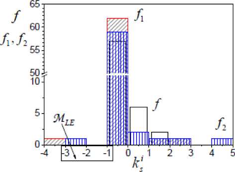
Fig.2. Bar chart of distribution simple roots system of the third order

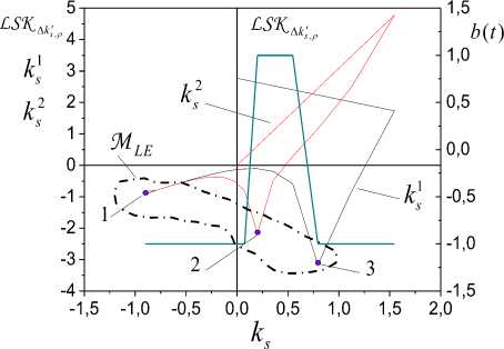
Fig.1. Estimation of an order and roots of the system of the third order

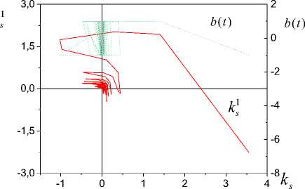
Fig.3. Estimation of roots for system of the second order with imaginary roots

of the structure SK ' about a coordinate origin. It is an ks, P indication of imaginary roots. On a bar chart (Fig.4) the largest LE is equal to null. It coincides with system parameters.

The method of an estimation an imaginary part roots by means of secants is described in [14].

On Fig.5 we will show results of identification system the second order with complex roots

A =

- 2 - 2

, O (A ) = ^{( — 1} + i , ^{— 1 —} i )

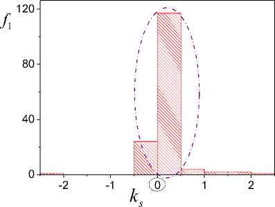
Fig.4. Distribution of imaginary roots system the second order

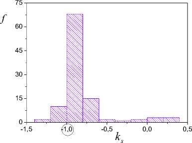
Fig.6. Frequency function of distribution values imaginary roots

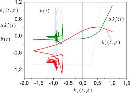
Fig.5. Structures for an estimation of an order of system with complex roots ( m = 2 )

We showed on Fig.3 results of identification a spectrum eigenvalues system (1) second order with ( A ) = ( - 2 i ; 2 i ) . The input has a sinusoidal form. It gives condition fulfilment h -identifiabilities. We will not show a matrix of a condition A of the system. On the base < r ( A ) obtain a Frobenius matrix not a problem. From the Fig.3 we see that the system has no real roots. The system order is equal to two. We observe oscillations

The analysis of a change a function b ( t ) gives an estimation of an order system m = 2 . We about the value k ( t , p ) = - 1 (corresponds to value of a real part of a root) observe oscillations with decreasing amplitude. So, the structure LSK^  confirms presence of complex roots.

Distribution function of values k shows on Fig.6. It confirms the presence of a complex root and will show oscillations about value -1.

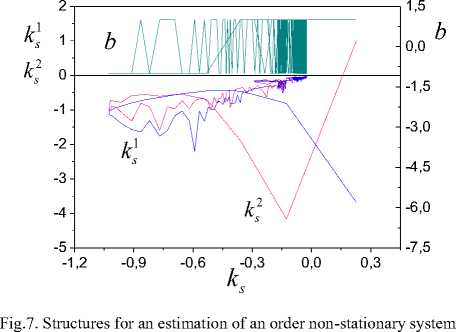
On Fig.7 show results of identification eigenvalues non-stationary system of the second order with

0 a ₁( t )

1 a ₂( t )

a_Y ( t ) = - 3 + 0.2sin(0.02 ^ t )

а_г ( t ) = - 4 + 0.3sin(0.04 ^ t )

Spectrum ст ( A ) = ( [ - 1.32; - 0.81],[ - 3.47; - 2.38] ) . The analysis of a variation the function b ( t ) gives an estimation of an order system m = 2 . On Fig. 7 we use the same designations, as on Fig. 1. The analysis of change functions k ¹( t ), k ²( t ) will show that we can obtain estimations for largest LE. Obtain for ^ an interval estimation [ - 0.89; - 1.14]. Mean value ^ on the interval is -1. The obtained results explain that the pyramid L ² ( t ) has no fixed steps. It does not allow to obtain constant value of an eigenvalue for pyramid steps. The structurally-frequency method gives a Perron bottom indexes as - 3.68 . This estimation is underrated. But the given method confirms its existence. We have offered an explanation of the obtained results. Therefore, the offered methodology for the considered class systems should be in addition researched.

We do not present results of an application of the procedures offered in section 8. They are considered in [14, 27]. Construct model for a variable y ˆ for check of the obtained spectrum ст ( A ) and estimate its adequacy. Ap-

ˆ ply static model the class of functions eJ and to estimate its adequacy.

Results of simulation confirm efficiency of the offered methods, structures and procedures.

• XII.    Conclusion

The approach to structural identification of linear dynamic systems on the basis of the analysis Lyapunov exponents in the conditions of uncertainty is offered. The method of deriving the general solution of a system on the basis of an application a static model is developed. The coefficient of structural properties of a system for an estimation of Lyapunov exponents is used. The special structures reflecting change LE, on the basis of a coefficient of structural properties, are introduced. The criterion of an estimation of an order of a system on the basis of the analysis of behaviour of these structures is offered.

In work is offered two approaches to an estimation of the largest Lyapunov exponent and the Perron bottom indexes. The first approach to identification of a change in a coefficient of structural properties with the help secant method for various classes of roots is grounded. The second approach is the structurally-frequency method grounded on obtaining of estimations indexes Lyapunov and Perron by means of the analysis of local minima of structures offered in work. The frequency method which is a modification of a method a bar graph in the statistical theory is applied to a validation of the obtained estimations. Results of simulation confirm effectiveness of the offered methods, structures and procedures.