Supercomputer simulation of oil spills in the Azov Sea

Recently, increase in oil production led to increase in emergencies associated with oil spill during transportation both by vessels and through the oil pipeline in Russia. Among sources of oil pollution, we note river runoffs, wastewater from enterprises located in coastal zones, drilling mud and sludge discharges at oil and gas well drilling, dumping of polluted bottom sediments of port zones, atmospheric precipitation and aeolian depositions. The oil has a toxic effect on phytoplankton at concentrations of 10 ^-8 – 10 ^-3 mg/l (cell division slows down or stops, the main production decreases). If the oil concentration is 0,05 – 0,5 mg/l, then primary production of marine phytoplankton is reduced to 50%.

Among the most well-known programs for predicting the oil spill spread in water, we note the “Green Sea Ranger” model of the “Korea Research Institute of Ships and Ocean Engineering” ; application programs (SHIO, OSSM, CATS, GNOME Analyst) of the US Agency “National Oceanic and Atmospheric Administration” (NOAA); the “Seatrack the Web” interactive numerical model of the Swedish Institute for Meteorology and Hydrology (SMHI). However, many models represent oil slick distribution, which is in agreement with real situation only at the initial stages of spill.

Analysis of numerical solution to the material transport model problem shows that time costs are reduced, then the grid dimension of explicit scheme increases. Modification of the explicit scheme using the parameter-regularizater can simplify the restrictions on the permissible value of time step [3]. In addition, explicit regularized schemes show the time advantages (10 – 15 times and more) in contrast with the previously used conventional implicit and no-regularized explicit schemes [4]. In the case of filling control domains, the variation of the finite volume method was proposed in [5, 6]. Algorithm of calculation taking into account the partial “fillness” of cells without flows is associated with a stepwise representation of a boundary on a rectangular grid. The proposed method was applied to solve three-dimensional hydrodynamic problems [7–9].

1.    Problem Statement

The complex of interrelated mathematical models of hydrodynamics and biological kinetics was used for mathematical modelling of oil destruction processes. Flow fields, used for calculation of the oil products transport, was calculated on the basis of this model.

• 1.1.    Mathematical Model of Hydrophysics

The initial equations of hydrodynamics of shallow waters are as follows [10, 11]:

– the motion equation (the Navier–Stokes motion equation)

u t + uu x + vu y + wu z = ^— pp X + (^u X ) X + ( pu y ) _y + ^(vu z ) Z + 2^Q( v sin ^{0 —} w cos⁰),

— 2Q u sin 0,

v t + uv x + vv y + wv z = P y + (^v x ) X + (Ry ) _y + ^{( v}v z )Z ^— 2^ u ^{sin 0},        ⁽¹⁾

1 ^p ‘

w t + uw x + vw y + ww z = P z + ⁽Pw x)x + (^wy) _u + ^(vw z X + 2^ u ^{cos 0} + g ⁽ P 0 Ip ^— 1) ; ^ρ

• – in the case of variable density, the continuity equation

• ^p t + ⁽pu) X + ⁽ p^{v )} y + ⁽pw) Z =⁰,                             ⁽²⁾

where u = (u, v, w ) is a velocity vector; p is an excess pressure above the undisturbed fluid hydrostatic pressure; p is a density; Q is an Earth’s angular velocity rotation; 0 is an angle between the angular velocity vector and the vertical vector; p, v are horizontal and vertical components of the turbulent exchange coefficient, respectively.

Consider system of equations (1), (2) with the following boundary conditions:

– at the input (the mouth of Don and Kuban rivers), u = uo, pX = 0,

– on the lateral boundary (beach and bottom),

P v P ^{( u} t ) ‘_n = ^{— T} , ^u n = 0, P X = 0

– on the upper boundary,

PP ⁽ u T ) ‘ n = ^{— T} , ^w = ^— ^ ^— p t /pg, ^p n = 0,                    (3)

– at the output (Kerch Strait), p'n = 0, un = 0, where n is the outer normal vector to the boundary of the computational domain; un, uτ are the normal and tangential components of the water flow velocity vector; pn is the normal component of the pressure over hydrostatic pressure; ω is the liquid evaporation intensity; т = {тх,Ty,Tz} is the tangential stress vector (Van-Dorn law); pv is the suspension density.

For the free surface, the tangential stress vector is defined as т = paCds |w| w, Cds = 0, 0026, where w is the vector of the wind speed relative to water; pa is the density of the atmosphere; Cds is the dimensionless surface drag coefficient, which depends on the wind speed and is considered to be in the range 0,0016 – 0,0032.

In these terms, we can rewrite the tangential stress vector for the bottom as т = pCd b | u | u ,Cd b = gk/h ¹ / ³ , where k = 0, 04 , k is the group coefficient of roughness in Manning’s formula, k E [0,025, 0,2] ; h = H + n , h is the total depth of the water area, [m]; H is the depth to undisturbed surface, [m]; η is the height of the free surface relative to the geoid (Sea level), [m].

On the basis of the measured velocity fluctuations, the discussed below approximation is required to develop the coefficient of vertical turbulent exchange, which is heterogeneous in depth [6]:

v = '^■« where U, V are the time-averaged pulsations of the horizontal velocity components; A is the grid scale; C s is the dimensionless empirical constant, whose value is generally determined by calculation of the decay of homogeneous isotropic turbulence. The grid method is used to solve problem (1) – (4) [12]. The approximation of equations by the time variable is performed by splitting schemes into physical processes [13] using the pressure correction method.

• 1.2.    Mathematical Model of Oil Spill Transport

The following system of equations is used to describe the process of oil products transport, which is subject to the evaporation of light, neutral and no-evaporating pseudofractions of oil spot, dissolution of oil slick and biodegradation [14–17]:

( c i ) t + u(c i ) x + v ⁽ c i ) y = O*(c i ) X ) X + ⁽^*( c i Y y ) y ^{— a} i ⁽ T ) ^— Mc i ) M          (5)

Mt + (u + Um )Mx + (v + vm )M'y = (^MX )X + (цМу )y + Ym (ci )M — AM, (vi )t + u(Vi )X + vM + «Nz = (X^iDX + WviYy )y + (M*(^i )Z )Z, (ci)n |(x,y)GY = 0, Mn |(x,y)GY = 0, (vi)n | (x,y,z)er\(z=G) = 0, (VYz |(z=0) = 0, where ci is the concentration of the i-th oil fractions, i = 1,k; рш,p are the water and oil density, respectively; ^* = ^ + (p — рш)gh3/^ is the function describing the pollutant

l decomposition process; ^ is the diffusion coefficient; g is the acceleration; h = ^ ci is the width of oil slick; αi , βi are the coefficients taking into account the decrease in light oil fraction concentration due to the evaporation, dissolution, and bacterial decomposition; M is the concentration of microorganisms; uM = (uM ,vM ),uM vVM are the components of microorganism velocity relative to water; YM = YM(ci,T) is the velocity of microorganism growth; λ is the rate of cell death; ϕi is the concentration of the i-th oil fraction in dissolved state, i = k + 1, l.

Changes of the oil solubility are described by the equation

Si = Sioe-0^, where Si0 is the initial oil solubility; t is the time, [day]. The coefficient of horizontal turbulent diffusion depends on hydrodynamic and climatic conditions under which the process takes place. The coefficient of horizontal turbulent diffusion is subject to the “four thirds” law of Richardson under difficult hydrodynamic and climatic conditions of the Azov-Black Sea area [1, 14]:

µ ≈ ε ^{1 / 3} L ^{4 / 3} ,                                           (6)

where L is the characteristic size of diffusing spots; ε is the rate of turbulent energy dissipation, which has the order 10 - 1 — 1 cm ² /s ³ at the surface and is reduced to the order 10 - 4 — 10 - 3 cm ² /s ³ at the average along with depth. For the one-shot volley oil spill, the following boundary and initial conditions are determined to solve the above systems of equations:

ci |t=0,(x,y)eA = ci0, ci |t=0,(x,y)^A = 0, where A is the area covered by the spot; ci0 is the oil concentration in the considered area.

• 1.3.    Modelling the Microbiological Destruction Processes of Oil and Oil Products

In order to research the bioremediation processes of oil slick including the evaporation, dissolution, biological oxidation by microorganisms, we endow system (5) with the functional dependencies (observation models) y (c i ) = ^ _m c _i /(c _i + K s ) , where ^ m ( T,C,I ) is the maximum velocity of microorganism growth; T is the ambient temperature over the spill surface; C is the water salinity; I is the water illumination; K S is the saturation coefficient; a i ( T ) = ( K e P i / ( RT ) + K D S i ) AX i M m , K e = 2,5 • 10 - 3 U 0 , 78 is the mass transport coefficient for hydrocarbon, [m/s]; U is the wind velocity relatively to water, [m/s]; X _i is the mole fraction of the i -th component equaled to v i / v i ; v i is the amount of the i -th component substance, [mol]; P i is the vapor pressure of the i -th component, [Pa]; R is the universal gas constant, R = 8, 314 J/mol; A is the area of oil spill, [ m ² ]; M im is the molar mass of the i -th component, [kg/mol]; K D = kK D ₀ is the coefficient of mass transport of dissolution; K _{D 0} is the initial value of the mass transport coefficient of dissolution; k is the coefficient depending on the water situation; S i is the dissolubility of the i -th component in water, [ kg/m ³ ]; ^ _{i 0} = K D SiX i M im ; в г ( c i ) = Y(c i )/q , q is the proportion coefficient between the amount of microorganisms and the absorbed substrate.

We endow system (5) with the equation [18]

= ^⁽u M ) x) + ^⁽uM^

(u _M ) t + (u + u m ) ( u m ) X + (v + v m ) ( u m ) y

— a u U M + k i grad c i ,

where M is the microorganism concentration (bacteria); αu is the coefficient of microorganism inertial motion; ki is the taxis ratio.

In order to research the microbiological oil destruction process, we simulate the introduction of biosorbent containing oil-oxidizing bacteria and the concentrated culture of the Chlorella vulgaris Beijer green microalgae. The coefficient λ takes into account not only the mortality of phytoplankton, but also the consumption of the phytoplankton by fish. We endow system (5) with the following two equations:

S t + uS X + vs y + wS Z = ^S ) X + (^s y ) y + ^S ) Z — (a o + YB W + D(S p — S ) + f,

B ‘ + uB'x + vB’ + wB’ — (^B ‘ )ж + (^By )y + (^B()‘ + kDM — cB, x y z xx yy zz where S, B are the concentrations of nutrient and metabolite of the Chlorella vulgaris Beijer green algae, respectively; a = (a0 + yB) is the growth dependence (the phytoplancton) due to the coefficient B ; α0 is the growth rate of M in the absence of the coefficient B; Y is the impact parameter; 5 = 5(C) is the loss coefficient of phytoplankton due to the extinction (specific mortality), taking into account the influence of salinity C; D is the specific pollutant rate; f (x,y,z,t) is the source function of pollutants; Sp is the maximum possible concentration of pollutants; kB is the excretion rate; ε is the metabolite decomposition of the coefficient B; ^(I,T, S,C) is the coefficient taking into account the effect of light, temperature, S and C on M .

2.    Method to Solve the Model Problems

In order to implement the oil product transport model, consider the two-dimensional convection-diffusion problem in the form ct + ucx + vcy = (^cx)x + (^cy )y + f                        (7)

with the boundary conditions cn(x,y,t) = an c + вп,                               (8)

where u, v are the water velocity components; µ is the turbulent exchange coefficient; f is the function, describing the intensity and distribution of sources; α n , β n are the given coefficients.

Introduce the uniform rectangular grid wh = {tn = пт, Xi = ihx, yj = jhy; n = 0, Nt, i = 0, Nx, j = 0, Ny,

NT = T,Nxhx = lx,Ny hy = ly}, where τ is the time step; hx , hy are the spatial steps; Nt is the upper time boundary; Nx , Ny are the spatial boundaries; lx , ly are the maximum dimensions of the computational domain.

For model discretization of the oil products transport problem, we use the space splitting scheme taking into account the partial filling of cells [12]. The discrete analogue of diffusion-convection equation (7) has the form

„ n+1 / 2 ^q i,j

^{n q} i,j

τ

⁺ ^ xL

n - 1 / 2 ^q i - 1 ,j

2t

n - 1 ^q i - 1 ,j

⁺ ^ xR

a n ^-1 / ² q i+1,j

2t

n - 1 ^q i +1 ,j

+ u

n qi+1,j

n qi-1j

4h _x

+

nn     n  n    n   nn

,      q i j     q i- 1,j      ,      q i+1j     q ij      о lex   q i+1j     ² q i j ⁺ q i- 1,j  I 1 /n / / n \ । n \

+ ^ xL U -j^ ---j + ^ xR U ---j---- j = 3/2^--- j----j------j + 1/2 (g(q nj ) + n nj );

h _x                  h _x                      h _x

n +1 ^q i,j

n +1 / 2 ^q i,j

τ

+ ^ yL

^q iⁿ,j - 1

n - 1 / 2 ^q i,j - 1

2t

+ ^ yR

n qi,j+1

n - 1 / 2 ^q i,j +1

2t

+ v

n +1 / 2 ^q i,j +1

n +1 / 2 ^q i,j - 1

+^yL V

n +1 / 2 ^q i,j

n +1 / 2 ^q i,j - 1

h y

+ ^ yR V

n +1 / 2 ^q i,j +1

n +1 / 2 ^q i,j

4 h y

+

= 3/2^.

n +1 / 2 q i,j+1

2C / ²

n +1 / 2

⁺ q ij - 1

h y

h 2 _y

+ 1/2 (g(qn.)+ n n₃ ),

where ^ xL = 1 , ^ xR = 0 for u> 0 , and ^ xL = 0 , ^ xR = 1 for u <  0 ; ^ yL = 1 , ^ yR = 0 for v > 0 , and ^ _yL = 0 , ^ _yR = 1 for v < 0 [11].

The research of scheme (9) shows that the scheme is stable at the Courant numbers in the interval [0; 0,75] and the large Peclet numbers ( Pe >20). In the limiting case (the diffusion coefficient is equal to zero) at large Peclet numbers, the maximum value of the numerical solution error of problem (7) obtained by proposed difference scheme (9) is equaled to 0,125. The numerical solution error obtained by scheme (9) is less than the solution error of problem (7) obtained by the discretization of standard difference schemes.

3.    Parallel Implementation as a Software Complex

Decomposition methods of grid domains are performed for computationally laborious convection-diffusion problems in parallel implementation taking into account parameters of multiprocessor systems’ architecture. The maximum performance of multiprocessor computer system (MCS) is equaled to 18.8 TFlops. As computational nodes, we use 512 single-type of 16-core Blade-servers HP ProLiant BL685, each of which has the four quadcore AMD Opteron processor 8356 of 2.3GHz and memory, which is equaled to 32 GB. Table 1 gives the time costs required for one time layer on various grids, as well as the acceleration and efficiency values for different numbers of MCS cores.

Table 1

Acceleration and efficiency of the number of processors ( p ) for one time layer

p	Computational domain	100 х 100	500 х 500	1000 х 1000	5000 х 5000
1	Time, s	0,000271	0,00846	0,03608	1,633
	Acceleration	1	1	1	1
	Efficiency	1	1	1	1
4	Time, s	0,000052	0,00341	0,00978	0,533
	Acceleration	5,212	2,481	3,689	3,064
	Efficiency	1,303	0,62	0,922	0,766
16	Time, s	0,000025	0,00054	0,00628	0,142
	Acceleration	10,84	15,667	5,745	11,5
	Efficiency	0,677	0,979	0,359	0,719
64	Time, s	0,000125	0,00016	0,00110	0,044
	Acceleration	2,168	52,875	32,8	37,114
	Efficiency	0,034	0,826	0,513	0,58
128	Time, s	^^^^^^^^^r	0,00040	0,00048	0,017
	Acceleration	^^^^^^^^^r	21,15	75,167	96,059
	Efficiency	^^^^^^^^^r	0,165	0,587	0,75
512	Time, s	^^^^^^^^^r	^^^^^^^^^r	0,00129	0,0072
	Acceleration	^^^^^^^^^r	^^^^^^^^^r	27,883	228,36
	Efficiency	^^^^^^^^^r	^^^^^^^^^r	0,054	0,446

For numerical implementation of proposed interrelated mathematical hydrophysics models, we develop parallel algorithms adapted for hybrid computer systems using the NVIDIA CUDA architecture (Fig. 1).

Fig. 1. The NVIDIA Tesla K80

The NVIDIA Tesla K80 computing accelerator has the high computing performance and supports all modern both the closed (CUDA) and open technologies (OpenCL, DirectCompute). The NVIDIA Tesla K80 specifications are the following: the GPU frequency of 560 MHz, the GDDR5 video memory of 24 GB, the video memory frequency of 5000 MHz, the video memory bus digit capacity of 768 bits. The NVIDIA CUDA platform characteristics are the following: Windows 10 (x64) operating system, CUDA Toolkit v10.0.130, Intel Core i5-6600 3.3 GHz processor, DDR4 of RAM 32 GB, the NVIDIA GeForce GTX 750 Ti video card of 2GB, 640 CUDA cores.

The GPU with the CUDA technology is required to address the effective resource distribution at solving the system of linear algebraic equations (SLAE). In order to implement the corresponding algorithm, we obtain the dependence of the SLAE solution time on the matrix dimension and the number of nonzero diagonals (see Fig. 2). As a result, in particular, we can choose the grid size and to determine the SLAE solution time based on the number of nonzero matrix diagonals.

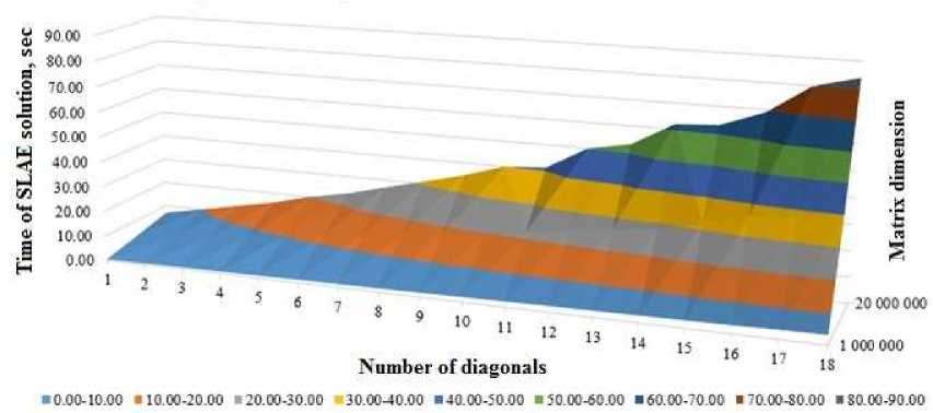
Fig. 2. Dependence of the SLAE solution time on matrix dimension and the number of nonzero diagonals

We implement the experimental software complex (SC) for mathematical modelling of shallow water ecosystems on the example of the Azov-Black Sea basin. Due to the SC, we can construct the operational forecast of movement of turbulence flow of water environment, i.e. the velocity field on grids with high resolution. The SC is used to calculate the three-dimensional velocity vector of the Azov Sea. The SC takes into account such physical parameters as the Coriolis force, the turbulent exchange, the complex geometry of bottom surface and coastline, evaporation, river flows, wind-surges, wind currents and friction bottom, and allows to calculate velocity field without pressure, hydrostatic pressure (used as an initial approximation for the hydrodynamic pressure), hydrodynamic pressure, and three-dimensional velocity field of water flow.

The output parameters are steps by spatial coordinates, error of grid equations’ calculation, grid dimension, time interval, evaporation intensity, initial distribution of velocity vector components of water environment and pressure.

We develop and integrate to this SC the new modules in order to calculate the oil products transport in view of the evaporation of light, neutral and no-evaporating pseudofractions of oil slick, dissolution and biodegradation.

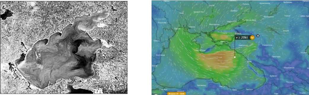
In order to calibrate and verify the developed hydrophysics models included in the SC, we use the “ESIMO” data [19] (Fig. 3), the NOAA data [20] (Fig. 4), and the “Analytical GIS” portal [21]. As input data, we use the NASA data [22], the Earth satellite sensing data of the Scientific Research Center (SRC) “Planeta” [23] (Fig. 5, 6), [25–29], the data of the Azov Fisheries Research Institute (“AzNIIRH”), the Federal State Institution (FSI) “Azovmorinformtsentr”, expeditionary researches [30, 31].

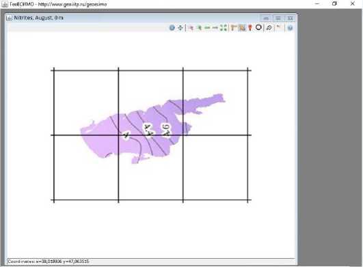
Fig. 3. “ESIMO” portal navigation panel that shows nitrites in the Azov Sea

a)                                            b)

Fig. 4. Earth satellite sensing data: a) the Azov Sea satellite image in ultraviolet spectrum (visible spots of phytoplankton, revealing the structure of currents);

b) the wind velocity and direction in the Azov-Black Sea basin

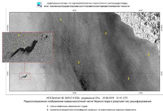
Fig. 5. SRC “Planet” data that gives description of oil pollution in the

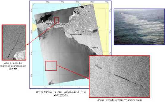
Fig. 6. IS3 Envisat radar image of oil slicks

Azov-Black Sea basin

The paper [10] gives the results of natural experiments for researching the crude oil destruction in seawater. According to the experimental results, only 3 – 15% of original amount of crude oil is subject to oxidation, biodegradation, photochemical reactions, while 10 – 40% of the substance is evaporated. According to the paper [24], the containment time should not exceed 4 hours since oil spill in water, and 6 hours since the discovery of oil spill on the ground for providing the information about spill upon receiving a message about spill.

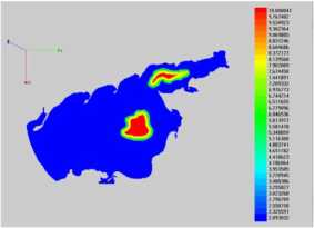
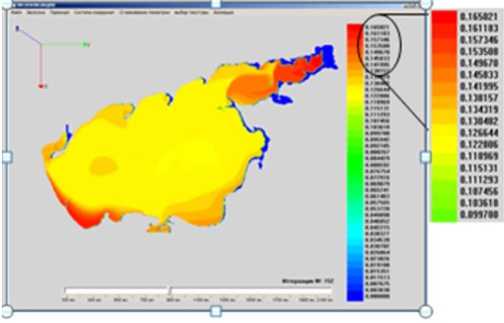
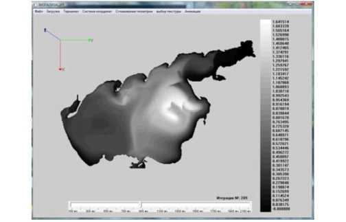
Fig. 7 shows numerical simulation of petroleum hydrocarbons’ bioremediation process by introduction of the in coastal system (the Azov Sea)   (N   is the

The initial distribution of light oil fraction is shown in Fig. 7 a, while the distribution of light oil fraction (two oil slicks) is shown in Fig. 7 b ( N = 121 ). The initial distribution of heavy oil fraction is shown in Fig. 7 c, while the distribution of heavy oil fraction concentration (a single localized spill with the subsidence of oil hydrocarbons to the water bottom) is shown in Fig. 7 d ( N = 148 ).

In the considered case, there is no localization measures of oil spills. According to the results

a)

c)

of natural experiments, the Fig. 7. Results of the

oil-degrading bacteria number of iteration).

b)

d)

“Azov3d” SC simulation

calculated time must be equal to 20 – 30 days. The wind velocity 3 – 8 m/s is an ideal for localization of the oil pollution. In this case, the slicks appear as dark spots on the bright (rough) water surface (see Fig. 8 a). The highest wind velocity was fixed in November 11, 2007 in Kerch Strait and amounted to 24 m/s according to the Gismeteo data.

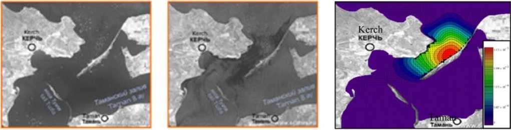
a)

b)

Fig. 8. Oil spill simulation using the “Azov3d” SC: a) the radar image during the spill;

• b) the concentration fields of light oil products

  Results of numerical experiments of light oil transport simulation in the Kerch Strait on November 16, 2007 (Fig. 8 b) was obtained on the basis of the developed SC and used to test the efficiency of this complex [26]. Compare the calculation results of the light oil product concentration (see Fig. 8 b) and the radar images of catastrophic oil spill (Fig. 8 a). Their qualitative agreement is obvious. The simulation time is 4 days after spill.

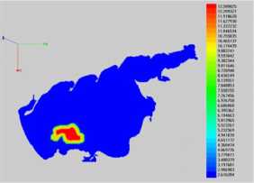
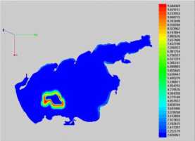
Simulation time interval was 30 days (Fig. 9 b). In the case of the source oil pollution (two oil slicks), the sorbed oil is reduced to 30 – 40%. This fact corresponds to the oil distribution process in water at the qualitative and quantitative levels. Fig. 9 shows the numerical simulation of the petroleum hydrocarbon phytoremediation process by the water algolization (the Azov Sea) with the Chlorella vulgaris Beijer green microalgae.

a)

Fig. 9. Results of “Azov3d” SC simulation: a) changes of biogenic pollutant concentration; b) changes of the Chlorella vulgaris Beijer green microalgae concentration (28 days since the introduction of algae in water). The coefficients are as follows: ^ = 5 • 10 - 10 ; D = 0, 001 ; S p = 1; f = 3 ; т ^ = 0,1; ^ e { M, S, B } ; e = 0, 8 ; a ₀ = 0,1 ;

Y = 0, 0416

b)

As the verification criterion of developed models (1) – (4), (5), we consider the error estimation of simulation taking into account the available field data measurements. The error is calculated as follows:

n

8 =. E(Cknat

k =1

^^^^^^^B

n

C k ) ² / л E

ck nat ,

k =1

where c k _nat is the value of harmful concentration obtained by field measurements [32]; c k is the value of harmful concentration calculated by the models (1) – (4), (5). The value of relative error δ was equaled to 12 – 24% at calculation of contaminant and microorganism concentrations.

Conclusion

We propose the complex of interrelated mathematical models of hydrodynamics and biological kinetics. The complex describes the oil products’ transport in view of evaporation of light, neutral and no-evaporating pseudofractions of oil slick, dissolution and biodegradation [30, 32]. The approximation of the convection-diffusion problem is performed on the basis of the space splliting schemes.

Research of the developed scheme shows that the scheme is stable at the Courant numbers in the interval [0, 0,75] and at the large Peclet numbers ( Pe >20). The proposed scheme gives the numerical solution error, which is less than the solution error of the problem obtained by the discretization of standard difference schemes. On the basis of supercomputer, we develop the experimental software for mathematical modelling the possible scenarios of shallow waters’ ecosystems on the example of the Azov Sea at oil spills. The decomposition methods of grid domains are used for computationally laborious convection-diffusion problems in parallel implementation taking into account the architecture of multiprocessor systems with distributed memory. Analysis of the CUDA architecture characteristics shows the applicability of algorithms for numerical implementation of the developed mathematical models of hydrophysics to construct the high-performance information systems.

Acknowledgements. This paper was partially supported by the grant no. 17-11-01286 of the Russian Science Foundation.