The Application of Sparse Antenna Array Synthesis Based on Improved Mind Evolutionary Algorithm

Author: Nan Li
Journal: International Journal of Intelligent Systems and Applications(IJISA) @ijisa
Article in issue: 3 vol.3, 2011.
Free access
Mind Evolutionary Algorithm (MEA) imitates the human mind evolution by using similartaxis and dissimilation operations, which overcomes the prematurity and improves searching efficiency. But the generation of the initial population is blind and the addition of naturally washed out temporary subpopulations is random. This paper improved MEA by introducing chaos and difference into it, which brought adequate diversity to the initial population and saved the excellent genes in the evolution. Then the improved MEA is used in the synthesis of sparse antenna arrays. The excellent results of computer simulation show the advantage of array antenna patterns synthesis using the improved MEA.
MEA, DEA, sparse antenna array, circular antenna array, side lobe level
Short address: https://sciup.org/15010183
IDR: 15010183
Text of the scientific article The Application of Sparse Antenna Array Synthesis Based on Improved Mind Evolutionary Algorithm
With the rapid development of the telecommunications industry, the electromagnetic environment of space is increasingly deteriorating, electromagnetic interference is enhancing and the quality of communication is declining. To solve these problems, smart antenna which has the ability of low side-lobes, strong directional and anti-interference has been a great deal of concern. The antenna pattern synthesis problem becomes a hot research. Antenna array synthesis means in a given antenna radiation pattern or antenna performance, design antenna array element number, element spacing, elements’ current amplitude and phase distribution.
The traditional numerical optimization method based on gradient searching technology is not effective enough for satisfactory results in project, because the objective function of antenna optimization problem is multiparameter, nonlinear, nondifferentiable and even discontinuous. Intelligent Algorithm has become a powerful optimization tool for its search does not depend on the gradient and search space information of specific problem.
Mind Evolutionary Algorithm (MEA) is brought forward by Professor K. M. Xie based on the analysis of human mind development and the imitation the similartaxis and dissimilation phenomena in human society [1]. But it also has some shortcomings. For example, the addition of naturally washed out temporary subpopulations is monotonous and random; the existing searching modes are easily to fall into local convergence. This paper integrated MEA with Differential Evolutionary Algorithm (DEA), and proposed Differential Mind Evolutionary Algorithm (DMEA). It introduced the thought of difference into the addition of naturally washed out temporary subpopulations. DMEA saved the excellent genes in the evolution and brought adequate diversity to the population. Compared with MEA, DMEA is more quickly, exactly and effectively, avoiding local convergence.
-
II. The Improved Mind Evolutionary Algorithm(IMEA)
A. Mind Evolutionary Algorithm (MEA)
The aggregation of all individuals in every generation in MEA is called a population; a population is divided into some subpopulations. There are two kinds in subpopulations: superior subpopulations and temporary subpopulations. Superior subpopulations record the winners’ information in global competition; temporary subpopulations record the middle process in global competition. The billboard provides the chance for the communication of the individuals and the subpopulations. There are three basic kinds of information in billboard: the sequence number, action and score of the individual or the subpopulation. The score is the valuation that the environment evaluates to the action of the individual or subpopulation. The individuals in subpopulations paste their information on local billboard. And the global billboard is used to paste the subpopulations’ information.
MEA inherited the idea of “population” and “evolution” from GA, but in other aspects MEA has big innovations. MEA divided a population into two kinds of subpopulations, superior subpopulations and temporary subpopulations. Superior subpopulations note the winners’ information in global, temporary subpopulations note the process of the global competitive. Firstly, MEA takes similartax operation on all the subpopulations and search optimal value in the local quickly by comparing fitness functions. Then dissimilation operation is used to search in the whole solution space, choice the better individuals as the centers and create new temporary subpopulations. Similartax and dissimilation both include choice operation. They repeat in turn in the evolutionary process. The individuals in the subpopulations post their information on the local bulletin board. The global bulletin board is used to post each subpopulation’s information.
Figure 1. Framework of MEA
B. Chaos Mapping
The chaos phenomenon is the common phenomenon in the nonlinear dynamic systems. The chaos’s behaviors are complex and similar to the random process, but have the inherent property of regularity. The chaos optimization algorithm is sensitively to the initial value, easily to jump out the local minimum, and quickly to search out the global optimization. It has the property of global asymptotical convergence [2-4].
Tent mapping is an important model of Chaos Dynamics with uniform probability density, power spectral density and ideal related characteristics. It is can be expressed as follow:
[2xk ,0 < xk < 0.5 x = k+1 [2(1 - xk ),0.5 < xk < 1
Its probability density function is:
P ( x ) = 1
Tent mapping has simple structure and good ergodic uniformity, more suitable for a large number of data processing sequences. But there are small iterative cycle and unstable periodic point in Tent mapping. It will make the iteration to the fixed point 0. In order to avoid iterates to fixed point, this paper uses the following method to improve Tent mapping:
x ( k + 1) =
x ( k )/0.4 x ( k ) < 0.4
(1 - x ( k ))/0.6 x ( k ) > 0.4
We can see that from Fig.1, the points generated by improved Tent mapping are scattered uniformly in [0.1]. It overcomes its own lacks, such as small cycle and instability cycle points.
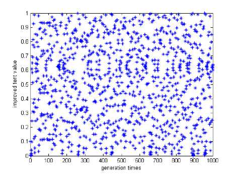
Figure 2. The chaos state of improved Tent mapping
C. Differential Mind Evolutionary Algorithm(DMEA)
In dissimilation operation of MEA, if the mature temporary subpopulation’s score is lower than any subpopulation, it will be abandon. And the search exploits new point to create new temporary subpopulation. But the creation of new temporary subpopulation is random and blind, lost the excellent genes in the evolution. This paper improved MEA for this shortcoming.
DEA is proposed by Rainer Storn and Kennth Price according to the evolutionary law of nature [5]. It is a real coding algorithm with simple configuration, quick convergence rate and strong stability. There are three kinds of operations in DEA: mutation, crossover and selection operations. And mutation operation is the key operation in DEA. In mutation operation, firstly select any two individuals in the population and compute their difference, then weight sum the difference and another individual to create new individual.
Let X, G , i = 1,2,..., N is the individual in generation G , G is the generation time, N is the population size. The new individual can be created by following:
V i,G + 1 = df ( Xr1,G - Xr 2, G )+ Xr 3 , G
(4) where r 1 , r 2 and r 3 are three different integers selected randomly in [1, N ]. df e [ 0,2 ] is the mutation factor to control the scaling of Xr^ G - Xr^ G .
D. The Improved Mind Evolutionary Algorithm(IMEA)
MEA simulated the similartaxis and dissimilation phenomenon in human society and resolved the problem of prematurity and low convergence speed of traditional Intelligent Algorithm to a certain extent. But it also has some defects. For instance, the generation of the initial population is blind and the addition of naturally washed out temporary subpopulations is random. This paper introduced improved Tent mapping and the mutation operation of DEA into MEA and proposed the improved MEA, which brought adequate diversity to the initial population and saved the excellent genes in the evolution.
The improved MEA is described as following:
Step1 Set evolutionary parameters: population size, subpopulation size and conditions for end;
Step2 Initialization: scatter individuals in terms of (3) in the whole solution space;
Step3 Similartax: individuals are produced by normal distribution with variance around each winner and the individual with highest score is the new winner replacing the old one in following steps;
Step4 Dissimilation: realize global optimization, some with lower score are washed out and replaced by new ones scattered according to (4) in the solution space;
Step5 Conditions for end: if the end conditions are filled, turn to step6; else repeat step3 and step 4;
Step6 Output evolutionary result, algorithm ends.
To assess the performance of IMEA, this paper selects three typical functions that commonly used to test optimization algorithm to experiment, which has multipeaks, non-raised and so on. The objective function is
F 1 = 100( x 12 - x 2 ) 2 + (1 - x 1 )2
-
- 2.048 < x 1 ,x 2 < 2.048
F 2 = ( 4 - 2.1 x 2 + x 4 /3 x 2 + X i x 2 + ( - 4 + 4 x 2 ) x 2 -10 < x 1 , x 2 < 10
sin2-i/I x ,2 + x 2 ) - 0.5
F 3 = : 1 8 2 ----\t - 0.5
[1.0 + 0.001 ( x 1 2 + x 2 ) ]
-
-10 < x 1 , x 2 < 10
F 1 is Rosenbrock function which has a global minimum. The global minimum position is (1, 1) and the value is 0. It is used to test the premature convergence of the algorithm. F 2 is Camel function which has six local minimums. The two global minimums are -1.031628, and their positions are (-0.0898, 0.7126) and (0.0898, -0.7126). F 3 is Schaffer function which has infinite local maximum . The only one global is maximum 1 and its position is (0, 0). The parameters of the experiment are: MEA and IMEA have the same large initial populations, the population size is 30, the subpopulation size is 18, the temporary subpopulation is 12, and termination time is 100.
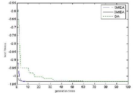
Figure 4. The convergence curve of Camel
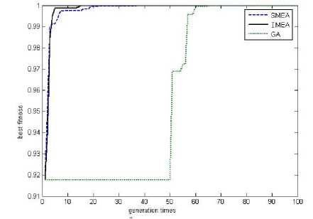
Figure 5. The convergence curve of Schaffer
TABLE I. Comparison of three functions’ optimization
RESULTS
|
function |
algorithm |
X1 |
X2 |
solution |
|
Rosenbrock |
MEA |
0.9947 |
0.9990 |
1.8231e-6 |
|
IMEA |
0.9996 |
0.9992 |
8.0936e-7 |
|
|
GA |
0.9091 |
0.8309 |
3.0325e-3 |
|
|
Camel |
MEA |
0.0899 |
-0.7122 |
-1.031625035 |
|
IMEA |
-0.0898 |
0.7126 |
-1.031628033 |
|
|
GA |
-0.0876 |
0.7106 |
-1.031600471 |
|
|
Shaffer |
MEA |
0.0066 |
-0.0030 |
0.9975 |
|
IMEA |
0.0014 |
-0.0001 |
0.9981 |
|
|
GA |
0.0098 |
0.0098 |
0.9975 |
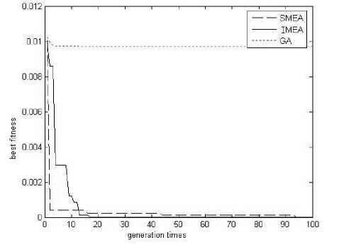
Figure 3. The convergence curve of Rosenbrock
From Fig.4-6 and Table 1, it can be seen in the three kinds of functions optimization, MEA and IMEA are effective. They are both able to find the optimal solution. From the solutions’ accuracy, the optimal values’ accuracy gained by IMEA is higher than those gained by MEA and the solutions’ positions are more accurately. This is because in different stages of the optimization process adopting different chaotic sequences to generate subpopulations. It’s not only to ensure the uniform distribution of the subpopulations and also improves the quality of the individuals. Thereby enhance the convergence of the algorithm and the accuracy of the optimal value.
-
III. sparse antenna array Synthesis
Antenna array is a kind of antenna consisted of some array elements to obtain special radiation characteristic.
According to the geometry structure, it can be divided into several categories: linear antenna array, rectangle antenna array and circular antenna array.
A. Uniform Linear Antenna Array
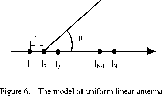
For a linear antenna array with given elements and spacing arranged in axis as it shows in Fig.6, its pattern formula is:
N
F V® ) = E I n exp [ j ( n - 1 ) kd cos 9 + V n ] (5)
n = 1
where I n is the n th element’s amplitude; v n is the n th element’s phase; 9 is the angle between the array axis and the ray; d is the space between the adjacent elements; k = 2л] A is wave number.
Let the antenna array’s main-lobe point at 9 0 , then V n = - ( n - 1 ) kd cos 9 0, (5) can be written as following:
N
F ( 9 ) = E I n exp [ j ( n - 1 ) kd ( cos 9 - cos 9 o )] (6)
n = 1
B. Uniform Circular Antenna Array
Antenna array is a kind of antenna consisted of some array elements to obtain special radiation characteristic, for example linear antenna array, rectangle antenna array and circular antenna array. Compared with linear antenna array and rectangle antenna array, uniform circular antenna array has bigger scanning range reached to 360° and counteracting mutual coupling effect with the symmetric uniform distribution.
As Fig. 7 shows, there are N elements distributing on a circle, R is the circle’s radius. 9 e [ 0, П 2 ] is the angle between signal incident direction and axis z , ф e [ 0,2 n ] is the angle between the direction that the signal incident direction projected on the xy plane. r = ( sin 9 cos ф ,sin 9 sin ф ,cos 9 ) is the direction vector and p n = ( cos ф „ , sin ф „ ,0 ) is the position vector.
Ф п = 2 n n / N is the n th element’s azimuth angle.
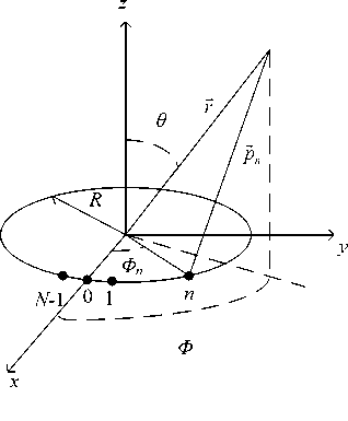
Figure 7. Uniform circular antenna array
The uniform circular antenna array’s pattern function is:
F ( 9 , Ф) =
N - 1
E
T p jVn - kR cos ( ф - ф и ) sin 9 ] I n e
n = 0
where In is the n th element’s amplitude and P n is
the n th element’s phase.
If let the antenna array’s main lobe point at ( 9 0, ф 0 ) , then P n = kR cos ( ф 0 - Ф п ) sin 9 0 , (7) can be written as
following:
N - 1
F ( 9 , ф ; 9 0 , ф 0 ) = E I ejltk R [ cos * * " ф " ) si n 91 - cos ( ф - ф " ) sin 9 ] (8) n = 0
If only considering the antenna pattern on the xy plane, then 9 = 9 0 = 90 0 , the pattern function can be written as
following:
N - 1
F ( ф ; ф 0 ) = E
T pjkR [ cos ( ф 0 - ф « ) - cos ( ф - ф „ ) ] n e
n = 0
C. Circular Sparse Antenna Array
In the engineering application of antenna array, narrow main lobe is often used to improve spatial resolution. To gain narrow main lobe in a full matrix antenna array, we have to enlarge the antenna array’s aperture. But it not only adds the cost but also increases the complexity of the antenna system. Distributing elements sparsely is another method to gain main lobe which saved the cost, improved the spatial resolution and avoided grating lobe.
Circular sparse antenna array has the big scanning range and high precision characteristics of circular array, and we can gain required antenna pattern by only optimizing the antenna array’s distribution. The pattern function is decided by the elements’ position parameter when optimize the antenna array’s distribution:
N f (9)=e e jkR [cos(90 - vn)-cos (9 - vn)] n =1
where 90 is the main lobe’s position, vn is the nth element’s azimuth angle, R = mA is the circular array’s radius, k = 2n/2 is wave number. In this paper m=2, (10) can be written as:
N
£ cos ( 9 0 - Ф п ) - cos ( e - Ф п )] + e j 4 n ( cos 9 o — cos 9 ) (11)
n = 2
D =
d 2
d 3
dN —1
x1 + dc x 2 + 2 dc
= X +
d c
2 dc
X N —2 +( N — 1 ) d c J [( N — 1 ) d c
= X + D C
For a linear sparse array with L = 9 Л , N = 10 , dc = ^ 2 ,
For a uniform circular full array, its element number is 24. Fig. 8 is the pattern of 24 elements circular sparse array and 12 elements circular sparse array.
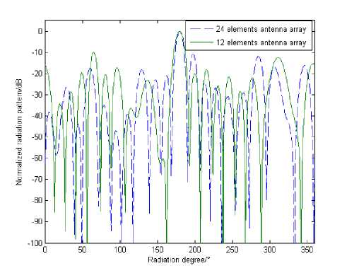
Figure 8. The circular random sparse antenna array
LZ = 9 ^ 2 , Dc = [ ^ 2, Л , 3 ^ 2,2 2 ,5 ^ 2,3 2 ,7 ^ 2,4 2 ,9 ^ 2 ] . We request the main lobe’s width is 5° and the highest side lobe level is -25 dB .
Different methods, GA and IMEA, were investigated and compared with simulation solutions in order to assess the effectiveness and the flexibility of IMEA. The experiment parameters of GA are: p c = 0.6, p m =0.1. The experiment parameters of IMEA are: df =0.5, the subpopulation size is 18, the temporary subpopulation is 12. In two algorithms, the evolutionary generation is 100 and the population size is 30. The simulation results are as following:
As Fig. 8 shows, the main lobe’s width of 12 elements array is similar to 24 elements array. It attests a circular sparse array with fixed radius can gain similar main lobe’s width with less element number, saving the cost. But the highest side lobe level of circular sparse array is high, the following optimization aimed at reducing the highest side lobe level of the circular sparse array.
IV. Simulation results
A. Linear Sparse Antenna Array
A linear sparse antenna array in fact is an unequal linear array with unequal space between the adjacent elements. Its pattern function can be written as following:
N
F ( 9 ) = ^ exp ( Jkdn cos 9 ) (12)
n = 1
where d n is the space between the first element and the nth element.
Before optimize the linear sparse array, we can pretreat the position variables to reduce the search range and improve the optimization efficiency [6].
Let the first element’s position variable is d 1 = 0, d c is the position variable’s difference between two adjacent elements:
min d - d j } > d c , 1 < j < i < N (13)
Then the left solution space is:
LZ = L — 2 d c — d c ( N — 3 ) = L — ( N — 1 ) d c (1
Scatter N -2 individuals composing initial population in the left solution space and sort them ascending to compose X = [ x 1 , x 2 , l , x N — 1 ] Г . Then the N -2 position variables in the linear sparse array can be written as:
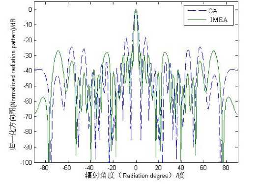
Figure 9. Optimization results of 10 elements sparse array for low SLL
TABLE II. Optimization results of linear sparse array elements’ positions
|
N |
GA |
IMEA |
||
|
X |
D |
X |
D |
|
|
1 |
0.2244 λ |
0.7244 λ |
0.3716 λ |
0.8716 λ |
|
2 |
0.7831 λ |
1.7831 λ |
0.6793 λ |
1.6793 λ |
|
3 |
0.8357 λ |
2.3357 λ |
1.2905 λ |
2.7905 λ |
|
4 |
0.9060 λ |
2.9060 λ |
1.5816 λ |
3.5816 λ |
|
5 |
0.9272 λ |
3.4272 λ |
3.0312 λ |
5.5312 λ |
|
6 |
1.0026 λ |
4.0026 λ |
3.2885 λ |
6.2885 λ |
|
7 |
1.0247 λ |
4.5247 λ |
3.7722 λ |
7.2722 λ |
|
8 |
1.1175 λ |
5.1175 λ |
4.0185 λ |
8.0185 λ |
From Fig.9, it can be seen that the highest side lobe level of GA is -20 dB , it does not satisfy the experiment request, while the highest side lobe level of IMEA reached -25 dB . From Table 2, we can see that the last element’s position variable is 5.1173 λ in GA while the last position variable is 8.0183 λ in IMEA when the solution space is [0, 8.5 λ ]. It shows the distribution optimized by
GA does not give full play to the advantage of sparse antenna array. It is most likely to get into local optimum.
B. Circular Sparse Antenna Array
For a circular sparse array, we can pre-treat the position variables to reduce the search range and improve the optimization efficiency.
The first element’s azimuth angle is ф 1 = 0 0 , ф с is the azimuth angle’s difference between two adjacent elements:
min ф i - ф j } > ф с , 1 < j < i < N (16)
Then the left solution space is:
LZ = 2 n - N ф c (17)
Scatter N -1 individuals composing initial population in the left solution space and sort them ascending to compose X = [ x 1 ,x 2 , l , xN - 1 ] Г . Then the N -1 position variables in the circular sparse array can be written as:
|
V = |
ф 2 ф 3 M |
— |
X i + Фс X 2 + 2 фс M |
= X + |
Фс 2Фс M |
= X + V c |
(18) |
|
V n . |
_ x N -j +( N - 1 ф _ |
.( N - 1 фс , |
For a circular sparse antenna array with R = 2 2 ,
N = 12 , ф с = П 12 , 9 0 = 0 0 , then LZ = 2 n - 12 \П 12 ) = n . We request the main lobe’s width is 20° and the highest side lobe level is -20 dB .
Different methods, GA and IMEA, were investigated and compared with simulation solutions in order to assess the effectiveness and the flexibility of IMEA. The experiment parameters of GA are: p c = 0.6, p m =0.1. The experiment parameters of IMEA are: df =0.5, the subpopulation size is 18, the temporary subpopulation is 12. In two algorithms, the evolutionary generation is 100 and the population size is 30. The simulation results are as following:
'^O 50 100 150 200 250 300 350
Radiation degree/0
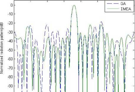
Figure 10. Optimization results of 12 elements sparse circular array for low SLL
From Fig.10, it can be seen that the highest side lobe level of GA has been reduced 6dB compared with Fig. 9., but it does not reach -20dB, while the highest side lobe level of IMEA reached the experiment request.
Figure 11. The polar pattern gained by IMEA
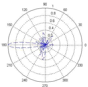
Figure 12. The polar pattern gained by GA
Fig.11 and Fig.12 are the patterns of the circular sparse array in polar coordinate optimized by IMEA and GA. We can see that there are only three side lobes whose normalized values exceeded 0.2 in Fig.11, while there are eight side lobes whose normalized values exceeded 0.2 in Fig.12. From Table 3, it can be seen that the last element’s azimuth angle is 208.64° in GA and the last azimuth angle is 345.00°in IMEA, while the solution space is [0°, 360°]. It shows the distribution optimized by GA does not give full play to the advantage of sparse antenna array. It is most likely to get into local optimum.
TABLE III. Optimization results of circular sparse array elements’ positions
|
N |
GA |
IMEA |
||
|
ψ c |
ψ |
ψ c |
ψ |
|
|
1 |
5.10° |
20.10° |
0° |
15.00° |
|
2 |
5.63° |
35.63° |
0° |
30.00° |
|
3 |
9.15° |
54.15° |
0° |
45.00° |
|
4 |
18.30° |
78.30° |
21.15° |
81.15° |
|
5 |
28.33° |
103.33° |
26.81° |
101.81° |
|
6 |
35.01° |
125.01° |
42.70° |
132.70° |
|
7 |
35.01° |
140.01° |
53.64° |
158.64° |
|
8 |
35.01° |
155.01° |
62.38° |
182.38° |
|
9 |
35.01° |
170.01° |
166.95° |
301.95° |
|
10 |
35.54° |
185.54° |
178.40° |
328.40° |
|
11 |
43.64° |
208.64° |
180.00° |
345.00° |
-
V. Conclusion
Point at the defects of MEA - the generation of the initial population is blind and the addition of naturally washed out temporary subpopulations is random. We introduced improved Tent mapping and mutation operation of DEA into MEA and proposed the improved MEA, which brought adequate diversity to the initial population and saved the excellent genes in the evolution. Then IMEA is adopted to optimize the linear sparse array and circular sparse array. There is a good agreement between the desired and calculated radiation patterns. And the optimizing result is better than that of GA.
References The Application of Sparse Antenna Array Synthesis Based on Improved Mind Evolutionary Algorithm
- K. M. Xie, Y. G. Du and C. Y. Sun, “Application of the Mind-Evolution-Based Machine Learning in Mixture-Ratio Calculation of Raw Materials Cement”, Proceedings of the 3rd World Congress on Intelligent Control and Automation, pp. 132-134, 2000.(in Chinese)
- K. Keiji, “Stability extended delayed-feedback control for discrete time chaotic systems”, IEEE Trans. On Circuits and Systems, vol. 46, pp.1285-1288, Oct 1999.
- L. Chen, G. R. Chen, “Fuzzy modeling, prediction and control of uncertain chaotic systems based on time series”, IEEE Trans. Circuits and Systems-I: Fundamental Theory and Application, vol. 47, pp.1527-1531, Oct 2000.
- R. L. Devaney, “An Introduction to Chaotic Dynamical Systems”, Addison-Wesley, 2nd ed, 1989, New York.
- R. Storn and K. Price, “Differential Evolution - A Simple and Efficient Adaptive Scheme for Global Optimization over Continuous Spaces”, Technical Report, International Computer Science Institute, vol. 8, pp. 22-25, Aug 1995.
- K. S. Chen, C. L. Han and Z. S. He, “A Synthesis Technique for Linear Sparse Arrays with Optimization Constraint of Minimum Element Spacing”, Chinese Journal of Radio Science, vol. 22, pp. 27-32, Feb 2007. (in Chinese)
- V. Murino, A. Trucco and C. S. Regazzoni, “Synthesis of Unequally Spaced Arrays by Simulated Annealing”, IEEE Trans. Antennas Signal Processing, vol. 44. pp. 119-123, 1996.
- B. P. Kumar and G. R. Branner, “Design of Unequally Spaced Arrays for Performance Improvement”, IEEE Trans. on Antenna and Propagation., vol. 3, pp. 511-523, 1999.
- K. S. Chen, Z. S. He and C. L. Han, “Design of Unequally Spaced Arrays for Performance Improvement”, Sensor Array and Multichannel Signal Processing, IEEE Workshop 2006, pp. 166-170, 2006. (in Chinese)
- E. M. Thomas and M. P. Krishma, “Pattern Synthesis of Conformal Arrays for Airborne Vehicles”, IEEE Aerospace Conference Proceeding, vol. 2, pp. 1030-1038, 2004.
- G. Caille, E. Vourch and M. J.Martin, “Conformal Array Antenna for Observation platforms in low Earth Orbit”, IEEE Antenna and Propagation Magazine, vol. 44, pp. 103-104,2002.
