The Image Recognition of Mobile Robot Based on CIE Lab Space

Published Online January 2014 in MECS

The development of the robot is to simulate human behavior ultimately. That is to say, it can sense the outside world. It also can solve problems that human can solve effectively. Humans can perceive the outside world mainly through sense organ such as visual, tactile, auditory and olfactory. At first, the information are gained from outside no matter there are humans or robots. Then the information is analyzed and extracted. Finally, it will make a response in order to achieve the desired purpose. According to human behavior, about 60% of the information are gained by visual. Therefore, it is crucial that the robot is given to the human visual function, which is an important way to take the initiative to obtain valid information for the robot.

Robot vision system is a biological science of visual function by computer simulation. Image processing techniques have been widely used in robot vision. As shown in Fig.1, the process of robot vision system includes image acquisition, the digitized image preprocessing, image segmentation, image extraction, and output results. Image segmentation is vital among them [1].

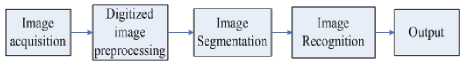
Fig. 1: Visual System Processes

Things around of Human perception are operated efficiently by the brain. So humans can make a meaningful response. We will take this process into the robot system. Today, CPU computing power has reached a stage of super-high-efficiency. It must be efficient and valid. It is the study of algorithms to solve the problem in order to avoid redundancy and duplication, and thus to achieve our purpose. This paper is simulate a space about robot vision system, as shown in Fig.2. There are some apples on the table and an apple photo on the wall. Our aim is to identify real apples. This paper presents two new algorithms. There are CIE Lab Space[2] and geometric deformation theory[3]. The algorithm is confirmed that it can identify real apples quickly and accurately.

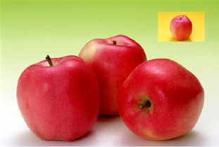
Fig. 2: Space Of Simulation

• II.    Digitized Image Preprocessing

• 2.1    MATLAB Software And Image Preprocessing

• 2.2    The Application of MATLAB in the Image

The robot collects digital images from the camera. The majority of these images exist geometric distortion due to the shooting angle of the camera. Dark current of camera CCD causes the image noise. Because of a variety of environmental factors around the robot, the digital image may have defects such as color cast and contrast. It is difficult to image recognition. Therefore, the images need to be preprocessed before image recognition. It can improve the image quality and eliminate the image noise. So image remains undistorted avoid blurring the edges of the image contours and lines. It also provide favorable conditions for effective image segmentation of the next step[4].

Image pre-processing technology is made before the formal processing of the image series of operations, because the image during transmission and storage process will inevitably be some degree of damage and a variety of noise pollution, resulting in deviation from the people's needs, which requires a series of preprocessing operations to eliminate the impact of the image. Overall image pre-processing technology is divided into two aspects, namely, image enhancement and image restoration techniques. Image enhancement techniques to account for a large proportion of the image pre-processing is a necessary step in the image processing, image restoration is to image restoration is to restore the original image of the essence for the purpose of image enhancement is based on the prominent people need characteristics and weaken the unwanted characteristics of the principle. Image enhancement method, there are many gray level transformation, histogram equalization, image denoising, pseudo-color processing. Gray-scale transformation is the basis and foundation of the image enhancement technology basically all image enhancement and gray-scale transformation. Image denoising, image enhancement, plays an important role in modern society. Fig3 shows the whole image preprocessing.

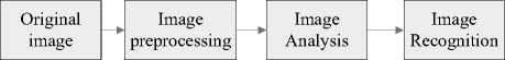
Fig. 3: Image preprocessing

MATLAB can be used for matrix operations, rendering functions and data, algorithm, creating the user interface, connect to other programming languages procedures. It is mainly used in engineering calculations, control design, signal processing and communications, image processing, signal detection, financial modeling, design and analysis and other fields. The most prominent feature of MATLAB is the simplicity. It's more intuitive accord with people instead of thinking of the code C and VC + + which is lengthy code. It brought us the most intuitive and simple program development environment.

• 1)    Image file format to read and write. MATLAB provides an image reading function imread (), which is used to read a wide variety of documents, such as bmp, pcx, jgpeg, hdf, xwd format images. MATLAB also provides image write functions imwrite (), in addition to the image display function image (), imshow ().

• 2)    Related to the basic image processing operations. MATLAB provides linear operation as well as an image convolution, correlation, filtering nonlinear operator. For example, it implements the A, B convolution operation of two images by the function conv2 (A, B).

• 3)    Image transformation. Image conversion image processing is an important tool. It is often used in image compression, filtering, coding and subsequent analysis feature extraction or message. MATLAB toolbox provides a common transformation functions, such as fft2 () and ifft2 () function. They can achieve twodimensional fast Fourier transform and its inverse transform, dct2 () and idct2 () function to achieve twodimensional discrete cosine transform and its inverse transform. Then Radon () and iradon () function can be achieved Radon transform and inverse Radon transform.

• 4)    Smoothing and sharpening filter. Smoothing techniques are used to analyze the noise in the smoothed image. It basically uses the averaging and median in the spatial domain. We usually think of the adjacent pixel gray very different point mutations as noise. Gray mutation represents a high-frequency component. Low pass filtering weaken the high frequency components of the image. It can be smoothed image signal. But it is also possible to make an image of the target area boundaries become blurred. The high-pass filtering method of frequency domain is used in the sharpening. It does this by enhancing high frequency components while reducing image blur, especially blurred edges are enhanced. But it also amplifies the image noise.

The above mentioned MATLAB in a variety of image processing applications are implemented through the corresponding MATLAB function. So we simply call the corresponding function correctly and enter the parameters.

• III.    Effective Image Segmentation and Extraction
  
  3.1    The Selection of the Color Space Model

• 3.2    Transformation between RGB Space and CIE Lab Color Space

Everything in the world can use mathematics to represent. We turn image into a mathematical formula (machine language) because of this feature. Then it can output the desired state through the calculation of the machine. We get relatively clear, undistorted image by preprocessing. The next step is to segment a valid image and extract it.

Each color space model has its own background and application areas. Color space model plays a decisive role in the selection of the segmentation results when the color image is segmented. Color image processing in the common color space includes RGB color space, HSI color space, CIE Lab color space and so on. According to trichromatic principle, RGB color space is established. It is the basic color space. It is also an additive color model. The three primary colors of red, green, and blue are summed in different proportions in order to produce a variety of color. The three primary colors are combined into a variety of different color light in each pixel from the full black to the full white. Each pixel is represented with 24 bits in computer hardware. Each of the three primary colors are assigned to 8-bit. According to the maximum value of 8 bits, each primary color intensity is divided into 256 values. 16,777,216 colors can be combined by using this method. But in fact human eyes can only distinguish the 1000 million colors.

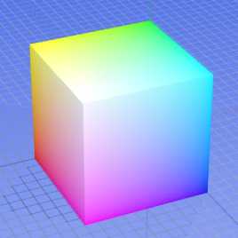
Fig. 4: RGB color space model

As shown in Fig.4, the color model is mapped to a cube. The horizontal X axis represents the red, which increases to the left direction. The Y-axis represents the blue, which increases down to the right direction. The vertical Z axis represents green, which increases upwards.

RGB space model is the basis of all color space model. Other color space model can be transformed through RGB space model. The color image is segmented by CIE Lab color space. CIE Lab color space has the advantage in that its color is closer to the human visual. This model focuses on perceptual uniformity. L ^* component exactly matches the brightness perception of humans. Therefore, we can modify the component and output levels of component for precise color segmentation. Contrast is adjusted by L ^* component. It is difficult to transform in the basic model. It is more important that the analysis of raw data is more realistic.

Transformation of the color space refers to transform the colors data of a color space into the corresponding data of another color space. That is to say, data in a different color space represents the same color. It turn the device-dependent RGB color space into the deviceindependent CIE Lab color space. Any devicedependent color space can be measured and calibrated in CIE Lab color space. The transition between them must be accurate if the color associated with the device can correspond to the same point of the CIE Lab color space.

Firstly, images must be converted to XYZ space from RGB space. Then it is converted to CIE Lab space from XYZ space[5]. As shown in Equation 1, the values of R , G , B are 0--100.

X ~	=     1	"  0.49	0.31	0.20  "	" R ~
Y		0.17697	0.81240	0.01063	G	(1)
	0.17697
Z J		[ 0.00	0.01	0.99 J	L B J

According to the calculation equation (2) of CIE Lab color space, we can get the component of the chrominance values of the color space.

' L = 116 f (Y / Y , ) - 16

• a * = 500[ f ( X / X n ) - f (Y / Y )] _ b * = 200[ f (Y / Y n ) - f ( Z / Z )]

f (t) = t1/3 when t > (6/29)3 in (2) , otherwise f (t) = 1(—)21 + 16/116 . The values of X„ , Y„, Z„ are 36                         n n n tri-stimulus values of the standard illuminant D65. As shown in Table 1, Xn = 95.04 , Yn = 100.00 , Zn = 108.89.

Table 1: The caption must be shown before the table.

	CIE 1913 2"
	x2	У2	X	к	z
A	0.44757	0.40745	109.85	100.00	35.58
D55	0.33242	0.34743	95.68	100.00	92.15
D65	0.31271	0.32902	95.04	100.00	108.89
F1	0.31310	0.33727	92.83	100.00	103.66

According to the (1) and (2), the RGB space is converted to the CIE Lab color space. we can obtain the equation (3).

• 'L* = 116(0.299 R + 0.587 G + 0.114 B )^1/3 - 16

a * = 500[1.006(0.607 R + 0.174 G + 0.201 B )^1/3 -

< (0.299 R + 0.587 G + 0.114 B )^1/3]                 (3)

• b* = 200[(0.299 R + 0.587 G + 0.114 B )^1/3 -

• 0.846(0.066G +1.117 B )1/3]

L ^* component is processed in adaptive brightness correction terms. Let the size of the input luminance of the image L ( i , j ) is M * N , the output image is h ( i , j ) , so it's transfer function is:

h ( i , j ) = <

h h  [ L ( i , j ) - L min ] + h a 1 , L min <  L ( i , j ) ^ L 1

"^1   ^min

^L ( i , j ) , ^L 1 <  ^L ( i , j ) ^ ^L 2

h - h

, b ² _"2 [ ^{L (} i , ^j ) ^{- L} 2 ] ^{+ h} a 2 , ^L 2 <  ^L ( i , ^j ) ^ ^L max

.^L max    ^L 2

A and B are the upper and lower limits of the average in the fruit under normal light image brightness statistical sample set. After a number of image analysis, the value is varied between 40-100: A and B are C component minimum and maximum of image brightness.

The image grayscale range is moved to the high when L _min<  L ( i , j ) < L in the (4). Pixels become lighter. Dark areas are stretched. It maintains when L <  L ( i , j ) < L . And the image grayscale range is moved to the low when L <  L ( i , j ) < L_{m x}. Pixels become darken. Bright area is compressed.

According to the selected transform function, the key is automatically selected the brightness of the image output range when segment transform boundary points are determined. It is determined that ( h a 1 , h_b 1 ) and ( h « 2 , h b 2 ) values. Using the following ways:

• 1)    Determine the brightness of image enhancement adjustment range:

According to Otsu (1979), brightness adjustment range is determined by the image in bright and dark areas between the maximum between-class variance. The total variance of the image is maintained because variance is a measure of the pixel gray level. Therefore, the discrimination of bright and dark areas is best when between-class variance is the maximum.

Let f (i, j) be a brightness value. B is normalized when the image L (i,j) at (i, j) (brightness value of

T = Averg L o mm < m — 1 ^a B ⁽ t ) J                         ⁽⁷⁾

In this way, we can determine the output image brightness adjustment range:

g a 1 = L min / T 1 , g b 1 = L 1 / T                   (8)

• 2)    Determine the brightness of the image reduced adjustment range:

• 3.3 Color Image Segmentation

We will distinguish defined as the maximum luminance value and minimum luminance value, the difference between the ratio of average worth. It is represented by T . Because the image grayscale range is adjusted from high to low.

T = (L - L / L                       (9)

2      max     min      mean

Therefore, the output image brightness adjustment range is:

g a 2 = L 2 / T 2 , g b 2 = L max / T 2                     (10)

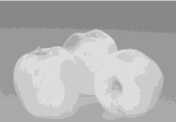
Fig.5 is collected in the original image. Fig.6, Fig.7 and Fig.8 correspond to the separation in CIE Lab color space of the L ^* channel, a ^* channel and b ^* channel. They are independent gray image.

each pixel is divided by 255). P ( i ) is the gray level for

the probability of k and it is denoted

^{P (} i ) = j^_ 1/ MN . Probability of bright areas

as is

t

Ю1 (t ) = ^ P (i)   . Bright regional average is i=1

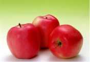
Fig. 5: Original image

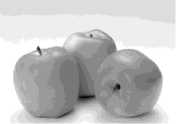
Fig. 6: ^{L *} channel

t

Ц 1 ( t ) = ^ iP ( i ) / Ю 1 ( t ) when the bright of image value is i = 1

t (0 < t < 1). Correspondingly, the probability of the dark m—1

region is rn ₂ ( t ) = ^ P ( i ) . Dark regional average is i = t + 1

m — 1

H 2 ( t ) = ^ iP ( i ) / ® ₂ ( t ) . Thus, the overall average of i = t + 1

*

Fig. 7: ^a channel

Fig. 8: b channel

image is:

P = ^ ( t ) p ( t ) + ® 2 ( t ) P ( t )                   (5)

According to the variance defined, we have:

^B ( t ) = ® 1 ( t ) [ A 1 ( t ) ^— a ] ² + ® 2 ( t ) [ Р г ( t ) ^— P ] 2       (6)

T

Thus, discrimination of bright and dark regions 1 is determined by:

CIE Lab color space is composed of threedimensional space according to the chrominance and luminance. It can be calculated for all light colors or object color. L* represents a lightness while a * and b ‘represent the chromaticity. But + a , — a , + b and — b respectively represent red, green, yellow and blue in the coordinate system. A component a * takes a value of —120 - +120 . The value of A component a* is usually displacement to 0 - 240 . so is b* . The lightness L* of the color is represented by a percentage. And it takes a value from 0-100.

a ^* channel is a monochrome channel. This method to gray image threshold segmentation is simple and effective. Fig.8 is a gray level histogram of the Channel a ^* . The horizontal axis represents the luminance value which is a total of 256 gray levels. In that case, 0 represents the darkest (black) and 255 represents the brightest (white). The vertical axis represents the number of pixels in each.

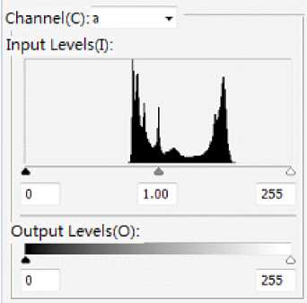
Fig. 9: Gray histogram of channel a ^*

According to the gradation of each pixel, the image is divided. Therefore, it is very important to how to determine the grayscale threshold. The threshold is too large or small to segment images accurately. OTSU method is considered the optimal method of the threshold selection[6][7]. So we choose equation (4) of the optimal threshold value.

T = max a2 (t)

= max { pi (t) p2 (t )[ц( t) - ^2 (t )]2}

p 1 ( t ) and p ₂( t ) are the probability of these two regions of the target and background after the threshold segmentation. ц 1 (t ) and ^ ₂( t) are the average grayscale value of these two regions of the target and background after the segmentation of the threshold value t. a ² ( t ) is square difference between the target and background class. t is the best segmentation threshold when a ²( t ) is the maximum.

According to the representation of a component information value, red and green are located at both ends of the shaft. Therefore, red and green is divided by the threshold value. The vicinity of the intermediate value of values represents a gradation value. Area which is higher than the value indicates the red. Pixels which a ^* component information value is greater than the threshold value T ₁ are considered to be red pixels. They set to 1 while the rest are 0. The red region r _red is obtained. Red apples are extracted by the equation (11).

r_red ( i , j )

Xzf [ r (i, j) < Ti] 0, else

Separated image r _red is a monochrome image of binarization. As shown in Fig.10, red apples as a white area while the remaining non-red background as a black region.

Fig. 10: The red area of a ^* component after segmentation

• IV. Discriminant Dimensional Objects

An object in the environment is a three-dimensional. An image is a two-dimensional object. We only need to increase a comparison sample image to judge an object is a three-dimensional or not. Briefly, we continue to have access to a same sample image from a different angle to compare with the original sample image. Flat or three-dimensional objects are analyzed through the sample image geometric principles. It is possible to confuse the effective information extraction when the ambient background is more complex. Thanks to this step, it can improve the accuracy of extraction of valid information.

In the example of Fig.2, there are two valid targets through the front of the color model. As shown in Fig.(11), next step is how to extract target 1 of true apples which are the three-dimensional image from target 2 of an image which is on the wall.

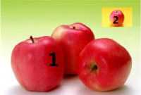
Fig. 11: Target 1 and target 2

We propose a new method---the secondary image sample collection. Specific methods are as follows:

First, we define the first collection of images for image samples 1 which have extracted the necessary information(Fig.12). Then a second image, which is defined image sample 2, is collected from different angles(Fig.13). We compare the image sample 1 and sample 2.

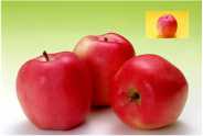
Fig. 12: Image samples1

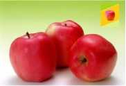
Fig. 13: Image samples2

Objects of sample 2 produce geometric distortion. There will be a different form for three-dimensional objects in a different location. Distortion of planar objects abide by the geometric principles[8]. It can be converted by a group of formulas. As a result, we can distinguish between three-dimensional objects and twodimensional objects based on the comparison of the two samples.

We use an algorithm to define the space transform. It describes how each pixel (image sample 1 ) moves from its initial position to the end position (image sample 2). This is the movement of each pixel.

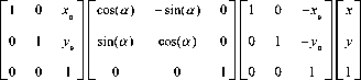
The spatial relationship between the sample 1 and sample II pixels is described by mathematical. Geometric operations in the general form of the space transform is defined as:

Equation (16) will produce a clockwise around the origin a angular rotation, which converted into a matrix form as follows:

a ( x , y )		cos( a )   - sin( a ) 0	x
b ( x , y )	=	sin( a )   cos( a )   0	y	(17)
_      1      _		_    0          0       1 _	_ 1 _

Summary, we obtain the equation (18):

a ( x , y )

b ( x , y )

g j ( x , y ) = f j [ a ( x , y ), b ( x , y )]                  (12)

f ij ( ^{x ,} y ) is a pixel location in the image sample 1. g ij ( ^{x ,} y ) is a pixel location in the image sample 2. Function a ( x , y ) and b ( ^{x ,} y ) uniquely describe the spatial transformation. So:

Then we simplify images into the many basic graphics area. It take the vertex when the object is a polygon. It take four points at the edge of the arbitrary to constitute a polygon if it is irregular in shape. This article select any four points of the edges of the painting apple. It is seen as a quadrilateral. Shown in Fig.14.

a (x, y) = x + x0 b (x, У) = У + У yo

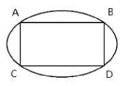
Fig. 14: Samples 1

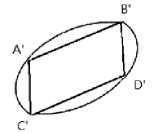
Fig. 15: Samples 2

Equation (13) is the translational operation of the pixel point. The moving distance of each pixel in the image is ^ x 2 + y 2 when f , (x , У ) is moved to the origin. Homogeneous coordinates are expressed that ^{x — y} is a three-dimensional space in a plane of z = 0 . So (7) is converted to a matrix form:

a(x, y) b(x, y)

10 xо x

01 y о y

1     0 0  11

If the spatial transformation:

/ x x

a(x, y) = -c b (x, y) = y

.        d

Equation (15) represents the image is enlarged c times in the X-axis direction while enlarged d in the Y-axis direction.

So:

a (x, y) = x cos(a) - y sin(a) b (x, y) = x sin(a) + y cos(a)

It abide by geometric distortion principle in transformation between sample 1 and sample 2 if the object is a two-dimensional plane. Each point comply with the space converting equation (19). It is only one. That is to say, the coefficient groups D¹ D ⁸ have corresponding equal.

"a ( x , y ) !  Г D 1 D ₂ D 3 D 4

b ( x , y ) = D 5 D 6 D 7 D 8

1         0  0  0  1

x

y

xy 1

The solution is obtained a set of coefficient values d i ^- D $ when it take A and A' into (19). Then it take B and B ^' into (19) result in a set of coefficient values D 1 ^- D 8 . It is consistent with the principle of plane geometry space conversion rules if these two sets of lines numerical corresponding equal. It conclude that this object is a two-dimensional planar object.

V. Agricultural applications

This paper technology can be widely used in agriculture. According to the different objects picking, picking apples and improve the image segmentation processing will require the majority of regional and even picking apples split the entire region. However,

due to the presence in the captured image old leaves, lesions on leaves and fruits, field other debris. Their color is similar. It would be mistaken as the goal. Target areas are some of glare. It makes the area look white to be mistaken for non-target areas. When Apple fruit with fruit character with different other colors, or surface debris covered by other colors. It is not able to pick apples are identified throughout the region. Therefore, we have to split the image after further processing. We will obtain a more complete objectives for the further provide conditions for the positioning of picking apples.

According picking apples target image color differences and background and objectives of the shape of the feature, we establish a picking apples identification method. In the selected color space, which can realize the accurate identification of apple picking the target image through the active partition and background. Experimental results show that the method of non-blocking picking apples ripe fruit has a better recognition results. It can better meet operational requirements. Since picking difference information and the background color is not only distinguished by the single color indicator, it is difficult to achieve a higher recognition rate. It will thus be increased by picking the object recognition method plurality of feature values. The method for the realization of apple picking job automation provides certain conditions, but also for other agricultural harvest automation, detection and classification provide a reference.

Analysis: The results generated misrecognized main reasons: a large portion of the captured image aperture adjustment will cause the image is overexposed 。 And backlit film will produce errors. Therefore, operations of agricultural should choose the right time for harvesting. So the effect will be better.

• VI. Comparison of the Calligraphic Character Skeleton Similarity

This article use CIE Lab color model of the image processing method to extract the color image objects accurately. It can distinguish between the threedimensional objects and two-dimensional objects through the secondary image samples collected contrast method and geometric distortion transformation principle in geometric space. The valid targets can be extracted efficiently and accurately because of the combination of the two algorithms. This method is simple and fast. Effective information is clear and accurate. And it is beneficial to the needs of the subsequent image processing. It is the clever that quickly distinguish different forms of the same object through samples contrast method in a complex environment.