Trajectory Tracking of Linear Inverted Pendulum Using Integral Sliding Mode Control

Published Online June 2012 in MECS

The linear IP system has the property of 4th order, unstable, multi-variable and highly coupled, which can be treated as a typical control problem to study modern control theories [1]. Since the control strategies of the inverted pendulum system is similar to the balance performance of the acrobats, and a lot of the abstract control concepts such as system stabilities, controllability, system anti-interference property etc can be displayed via the inverted pendulum system. The typical model of linear IP is shown in Fig.1 [2].

Controller design is the key content of linear IP systems. Controllers are used to stabilize the unstable system and make it robust to disturbances. Ample amount of research has already been done for the design part of controller and it is still challenging issue for the researches. It has been controlled by well known PID,

LQR, root locus, frequency response, fuzzy control, neural network, robust control, adaptive control and some more power algorithms which combine the above ones [2].

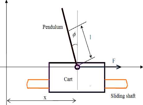
Figure 1. Model of linear inverted pendulum

Sliding mode control is an extremely robust control technique [3]. Sliding mode control is a special case from the theory of variable structure system.(VSS) The term VSS first made its appearance in the late 1950’s. It has been shown that dominant role in VSS theory is played by Sliding Modes, and the core ideal of designing VSS control algorithms consists of enforcing this type of motion in some manifolds in system spaces [4]. Traditionally, these manifolds are constructed by the intersection of some hyper surfaces in the state space and this intersection domain is normally called sliding surface. Once the state trajectory reach the sliding surface the structure of the system adaptively alter itself in such a way that the state trajectory slides along the sliding surface. This motion of the trajectory is called the sliding mode. During the sliding mode the system dynamics are governed by sliding surface dynamics giving completely robustness to the system against external disturbances and parameter variations. Sliding mode control design can be divided into two subparts viz. (i) the design of a stable surface and (ii) the design of a control law to force the system states onto the chosen surface in finite time. The design of the surface should address all constraints and required specifications therefore it should be designed optimally to meet all requirements. During the sliding mode the system is having order of n-m with n is the state dimension and m is the dimension of control input. Sliding mode control can give robustness to the system only if the states reach the sliding surface. The motion of the trajectory from the initial condition towards sliding surface until it hits the sliding surface and the condition for the sliding mode been satisfied is called the reaching phase. During the reaching phase, the system is sensitive towards the parameter variations and external disturbances as its motion is dependent on real system parameters and switching action based discontinuous control has not been started yet. So even matched perturbation can affect the system performance.

To solve the non-robustness nature of reaching phase an integral sliding mode concept has been proposed [5,6]. An integral term is incorporated in the sliding manifold, this guarantees that the system trajectories will start in the manifold right from the beginning thus, the reaching phase is eliminated; and the system becomes invariant towards matching perturbation right from the beginning. The main idea behind the ISM controller is to define the control law as a sum of a nominal control and a discontinuous control [7]. Unlike the sliding mode control the integral sliding mode control cannot be designed without using nominal control as the integral sliding manifold comprise of unknown initial condition. Nominal control takes care of the nominal plant dynamics and the discontinuous control rejects the disturbances [8]. The nominal control can be of any form which is able to follow the reference trajectory within a given accuracy.

Here the linearized model of Linear IP has been derived for the design of controller part. Linear IP has unstable equilibrium point in the vertically upward direction for which the control action is to be determined. The linearization has been done about that equilibrium point. The LQR control is designed as a nominal control for the linear model. However, while uncertainties exist, the system trajectory may deviate from the desired trajectory and the tracking performance would be deteriorated. When the control action from LQR controller is applied to IP system, it has to work with un-modeled dynamics and uncertainties as it is a complex system. This leads to deterioration of tracking performance and sometimes leads to instability. In this paper, the desired trajectory has been tracked considering linear model of IP using LQR controller and then additional control is introduced using integral sliding mode to ensure invariance against disturbances and stability with this combined control law is proved. The nominal control from LQR takes care of nominal plant dynamics and the discontinuous control from ISM takes care of uncertainties.

In this paper linear model for linear IP system is derived in section II. Sliding mode control techniques which have been designed already are analyzed in section III. Then LQR control and ISMC are explained in section IV. The ISM controller is designed to stabilize the pendulum and cart position in section V. In VI simulation results are presented which prove robustness of proposed ISM control scheme.

• II.    System Model

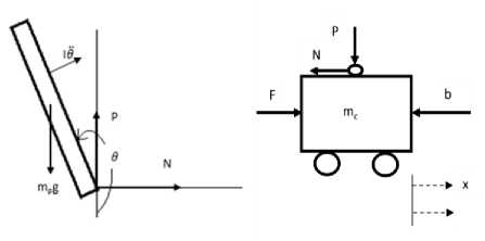
There are difficulties in IP system modeling because of its instability. But after ignoring some less important factors, the IP system becomes a typical rigid body in motion. The dynamic equation has been obtained in the inertial frame by classical mechanics theory. The objective is to balance the bob of the pendulum to a desired equilibrium point in vertically upward direction at reference position. The cart is driven by DC motor which is controlled by a controller (ISMC in our case). The current position of cart x and the pendulum angle φ are measured by sensors and supplied to controller to take control action. The Free Body Diagram of the system is shown in Fig.2 (a) and Fig.2 (b) to develop mathematical model. Here the air gap resistance and other frictions like cart and pendulum coupling, cart wheel and cart body etc. are ignored and the gravitational acceleration is assumed to be constant. The meaning and values of parameters are listed in Table-1.

(a)                             (b)

Figure 2. (a)pendulum force analysis (b)Cart force analysis

TABLE-1 Linear IP parameters symbols and values

Cart mass(mc)	1.096 kg
Pendulum mass(mp)	0.109 kg
Friction co-efficient of cart(b)	0.1N/m/s
Distance from pendulum rotation axis centre to pendulum mass centre(l)	0.25 m
Gravity acceleration(g)	9.8 m/s 2
Pendulum inertia(I)	0.0034 kg.m2

The variables are,

F - Force acting on the cart

• х - Cart position

φ - Angle between the pendulum and vertically upward direction

θ - Angle between the pendulum and vertically downward direction

The sum of forces acting in horizontal direction gives the equation of the motion mсẍ = F - bẋ - Ν          (1)

The force acting on the rod in horizontal direction is

N = m    (x + lsinθ)              (2)

From (1) and(2) the dynamic equation is obtained as

(mр +mс)ẍ + bẋ + mрlθ̈cosθ - mlθ̇ 2 sinθ = F(3)

The force acting on the rod in vertical direction is given by

P=mрg-mрlθ̈sinθ - mрlθ̇ 2 cosθ   (4)

The sum of the moments around the centre of the pendulum is given by

-Plsinθ - Nlcosθ = Ιθ̈                     (5)

From (4) and (5)

(I + mрl2)θ̈ + mрglsinθ = -mрlẍcosθ

Now from Free Body Diagram θ = π + φ;

To linearize the system near equilibrium point, assume          φ ≪ 1           ,           then cosθ = -1, sinθ = -φ and( )2 = 0. Here u is the input force.

From (3) and (6)

(mр +mс)x + bẋ - mр lφ̈ = u

(I +mрl2)φ -̈ mр gl φ = m р lẍ

From (8), expressing ẍ in terms of φ̈ , (7) is given by, ẍ =     ( I+mpP )" ẋ + φ+

(nip+тс)+ 1Пр1П^12     I(nip+тс)+nip тс12

( 1+тр12 )

I(Шр+тс)+ ГПрГПс12

From (8), expressing φ̈ in terms of ẍ, (7) is given by,

φ̈ =

-тр1Ь

I(Шр+тс)+ ГПрГПс12

ẋ +

m_pgl (тр+т_с) I(Шр+т_с)+т_рт_с1²

тр1

I(Шр+тс)+ ГПрГПс12

The state space equation can be written as, ẋ = Ax + Bu y = Cx+Du

Where

φ+

0      -(I + mр l )b

I(mр+m)+mрml

-mр lb

I(mр+m)+mрml

mр2 gl

I(mр+m)+mрml⎥

01⎥ mрgl(mр +m )⎥

I(mр+m)+mрml⎦

(I + mрl2)

I(mр +mс)+mрmсl2

0 mрl I(mр +mс)+mрmсl2

C=[

: ];D=[00]

The Eigen values of the system are 0, -0.0830, -5.2780 and 5.2726. Therefore it is unstable system.

With controllable matrix Cc=[B AB A2B A3 B], rank(Cc)=4;The observable matrix Oc= [C CA CA2 CA3 ] rank(Oc)=4.

So the system is controllable and external controller can be designed to stabilize the system.

• III.    Sliding Mode Control Analysis For Linear IP

Sliding mode controllers have been implemented successfully for linear IP [9-11]. Linear IP is a single input system so single control law must be derived to control the angle and position both together. Control of pendulum angle must be given higher priority than position control. Summing the two control actions does not give proper logic. Many researchers have developed the sliding mode control actions for controlling pendulum angle and cart position separately and then combined the two through some mechanism. In [9] signal selector switch has been used to select the control. When pendulum angle is within the threshold range, cart position control operates and if the pendulum angle cross the threshold value immediately pendulum angle control operates. In [10] the decoupled sliding mode control(DISMC) has been proposed in which the whole system has decoupled into two subsystems system A and system B. System A corresponds to pendulum angle control and sliding surface s1. System B corresponds to cart position control and sliding surface s2. The main target is to control system A. An intermediate variable z, which represents secondary information about s2 is incorporated to s1 and single control input has been derived which forces s1 to become zero first and then stabilizes s2. The derived single control input should be robust against the disturbance which is well known property for sliding mode controllers. The system has been tested for the response in the presence of sinusoidal disturbance. The simulation results have been shown in Fig.4 to Fig.7

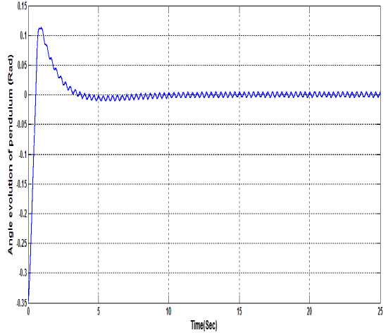
Figure 5. Angle evolution of pendulum in the presence of disturbance using Decoupled SMC

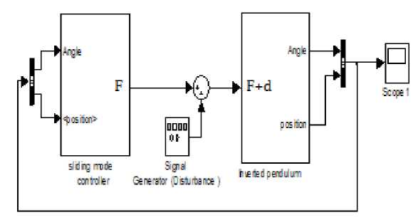
Figure 3. Simulink block diagram for decoupled sliding mode control in which the system is disturbed by disturbance signal d=0.5sin(t)

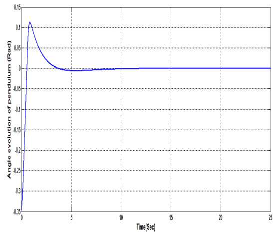
Figure 4. Angle of Pendulum using Decoupled SMC

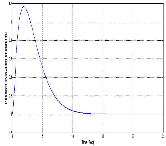
Figure 6. Cart position evolution using Decoupled SMC

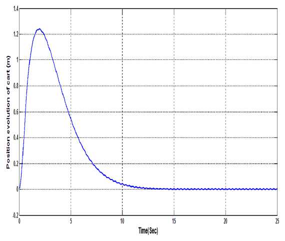
Figure 7. Cart position evolution in the presence of disturbance using Decoupled SMC

Fig.4 shows the performance of DSMC for pendulum angle control. Fig.5 shows the performance of DSMC in the presence of sinusoidal disturbance. Fig.6 shows the performance of DSMC for cart position control. Fig.7 shows the performance of DSMC for cart position control in the presence of disturbance. So we can say that the coupling of two control actions (angle control and position control) does not provide invariance against disturbance for which the SMC is attractive. So for tracking of desired trajectory of pendulum angle and position integral sliding mode control theory is applied to provide invariance against disturbances to system.

• IV.    LQR and ISM control

• A)    LQR CONTROL DESIGN

The LQR method is used to design a linear controller for a system with full state feedback. The LQR design method develops controllers of the form

x(t) = Ax(t) + Bu(t),x(0) = x ₀       (12)

x(t) e Rⁿ,u(t) e R ^m

A, В is stabilizable.

which minimize the cost performance

J = | j_o°°[x ^{T (}t⁾Qx(t) + u^T(t)Ru(t)] dt (13)

where Q is the symmetric, positive semidefinite state weighting matrix, and R is the symmetric, positive definite control weighting matrix. It is also necessary that [A,Q ¹ /² ] is detectable.

The solution of the regulator problem is a time varying control law which in steady state becomes the linear time-invariant, state feedback law[12],

u(t) = -Kx(t)

where K is the (m x n) control gain matrix given by

K = R" 1BTP

And P is the unique symmetric, positive semidefinite (n x n) solution of the algebraic Riccati equation

ATP + PA — PBR_ 1BTP + Q=0

The control law defined (14) is unique and minimizes the cost function, provided that the stabilizability and detectability conditions are met. If there are input disturbances to the plant, the optimal controller is determined as above, ignoring the fact that there are disturbances, and it is implemented as shown in Fig.8

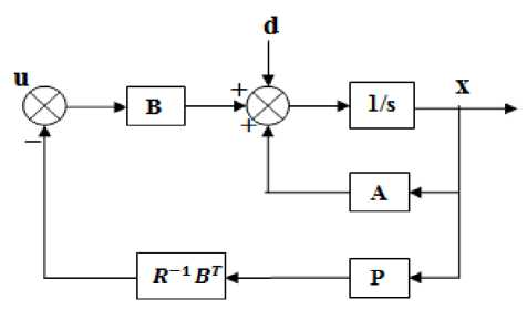
Figure 8.    LQR Implementation

The linear time invariant linear IP model in (11) is considered for LQR control design as, x (t) = Ax(t) + Bu0(t) ,x(0) = 0

y(t) = Cx(t)

u0 (t) is the nominal control from LQR.

The performance index is

J = ¹ J₀°°[e ^{T (}t⁾Qe(t) + Uo(t)Ruo(t)] dt (18)

where e(t) = r(t) - x(t)

The optimal control is designed that minimize the performance index which satisfies (15) and (16) is u0(t) = -Ke(t)

• B)    INTEGRAL SLIDING MODE CONTROL (ISMC)

The system in (11) with uncertainty and input disturbance is represented by x (t) = Ax(t) + Bu0(t) +d(x,t)      (21)

d(x, t) is the perturbation due un-modeled dynamics, and external disturbances which satisfies the matching condition in [9], that is,

d(x,t) = Bd _m                 (22)

and also |dm| < M,where M is a positive number determined by maximum bound of uncertainty. The control input for system in (11) is given by, u = u0 + u 1

Here u is nominal control input which can be designed by PID control, LQR control, pole placement or other control laws (In this paper it is LQR control). u is a discontinuous control which is designed to force the system to constrain state trajectory on the sliding surface and to eliminate the external disturbance. The integral mode sliding surface proposed in [5] is

s(x, t) =G{∫ ; (ẋ(τ) -ẋi(τ))dτ}         (24)

Here x(t) is the actual trajectory; xJ (t) is the desired trajectory given by nominal control in the absence of uncertainty and disturbances. Therefore, s(x, t) is the difference between the actual trajectory and desired trajectory projected on G. The projection matrix G is chosen in such a way that the Euclidian norm of resulting perturbation is minimal. It is reasonable to selectG = Β + , where Β +the left inverse of B. that is [6] is

Β+ =(ΒT Β)-1Β              (25)

From (12) and (16) the sliding surface is

s(x,t)=G{x(t)-x(0)-∫ ; (Ax(τ) + Βu0 (τ))dτ} (26)

where ∫ ) (Ax(τ) + Βu0 (τ))dτ is the desired is the trajectory; x(0) is the initial condition of the states. Thus ISM provides robustness to state trajectory from initial point. It is observed from (17) that in the absence of uncertainty actual trajectory exactly tracks the desired trajectory and sliding surface remains zero. In the presence of disturbance actual trajectory cannot track the desired one and sliding surface is having some nonzero value. Discontinuous control uses the value of s(x, t) to determine robust control action.

The objective of ISMC is to force the sliding motion on s(x,t)=0 , therefore it works as a disturbance observer and provides invariance against disturbances. Considering the Lyapunov function

V(x, t) =0.5sT (x, t)s(x, t)               (27)

The discontinuous control which satisfies V̇<0 is u!=-Msign(s(x, t)         (28)

• V.    Integral sliding mode controller design

  The structure of ISMC is shown in block diagram of Fig.9[4]. The weight matrix Q = diag[1000,0,400,0] and R=1 are chosen for system in (12) which satisfy (17). For that the gain value K from (11) is K=[-31.6228,-21.8547,85.1407,16.0398].

The nominal control from (15) is u0 = -Ke(t);

d = sin(2t) is chosen as disturbance. dm = 1. So M is chosen as 1.1. The gain value for the sliding surface is tuned to left inverse of the matrix B. That is G= [0,0.1394,0,0.3721] . The discontinuous control from (18) is u = -1.1sign(s(x, t)). The reference value is chosen for simulation results is x=1,φ=0.

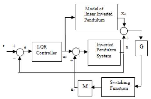
Figure 9. The block diagram of ISM control

The integral sliding mode control from (15) is

и ( t )=- Ke ( t )-1.1 sign ( s ( x , t )).

• VI.    Simulation Results1)    LQR control without disturbance(d=0)

It can be seen from Fig.10 and Fig.11 that when there is no disturbance present in the system the LQR control track pendulum angle and cart position accurately. This is the desired trajectory xJ (t) and because of no disturbance present, this is an actual trajectory x(t) also. The discontinuous control from ISM controller is zero.

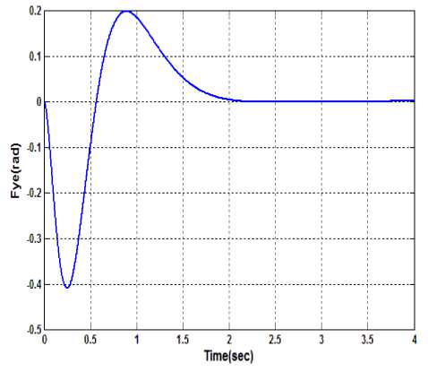
Figure 10. Pendulum angle evolution using LQR control

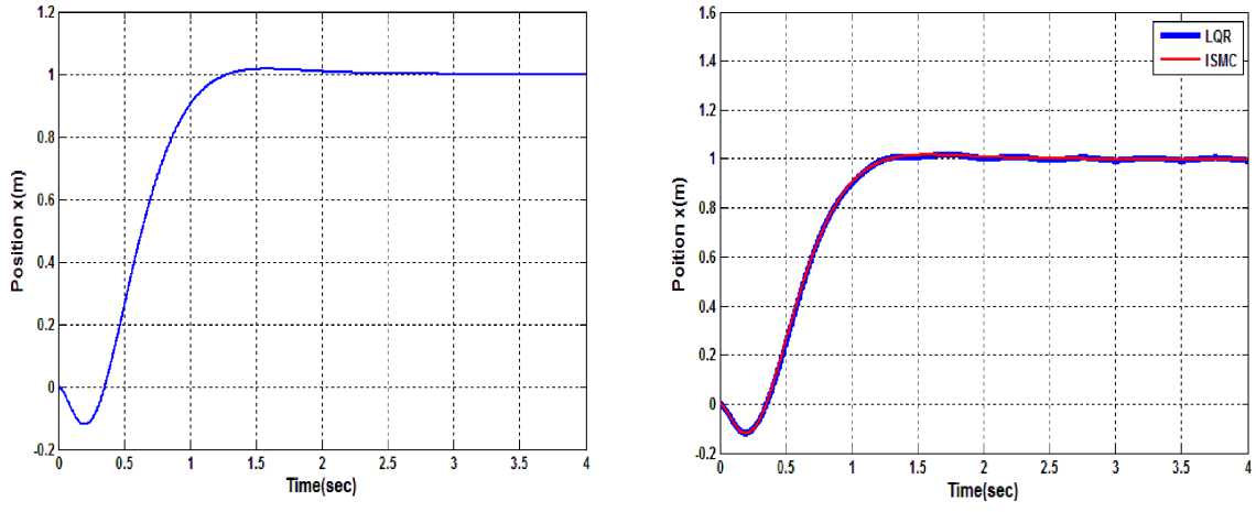
Figure 11. Position evolution of pendulum using LQR control

• 2)    LQR control and ISMC control with disturbance

The LQR control is tested for its disturbance handling capacity. The system is perturbed by sustained disturbance of sinusoidal nature d = sin(2t). It can be seen from Fig.12 and Fig.13 which show the plot of pendulum angle and cart position respectively for both LQR control and ISM control. The performance is dictated by the disturbance with LQR control. The amplitude of oscillation is increased as the amplitude of disturbance is increased. Whereas ISM control takes counter action and suppresses the effect of disturbance and provides the robust performance of the system.

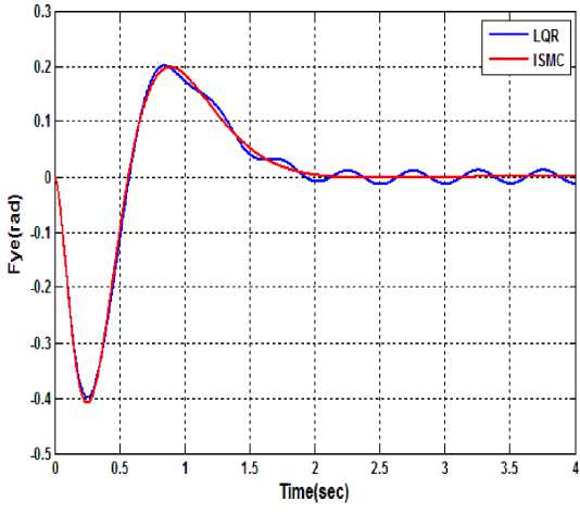
Figure 12. Comparison of angle evolution of pendulum in the presence of disturbance using LQR and ISM control

Figure 13. Comparison of position evolution of cart in the presence of disturbance using LQR and ISM control

Figure 14. Sliding surface evolution with time

«                      0.5                      1                      1.5                       1                      2.5 J 5.5                      4

Tme(sec)

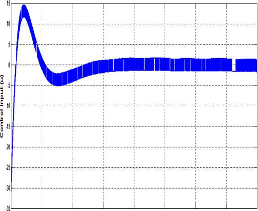
Figure 15. Input evolution using ISMC

Evolution of sliding surface with respect to time is shown in Fig.14. Here unlike SMC, s(x,t) remain in the vicinity of zero from initial time instant completely rejecting the reaching phase and ensures the robustness in the entire motion. The switching action starts in control input from the initial point showing the disturbance observer property of ISMC as shown in Fig.15.

• VII.    Conclusion

In this paper, an integral sliding mode control scheme is proposed to achieve trajectory tracking of linear inverted pendulum and simulation is done using MATLAB. The linearized mathematical model of linear IP is derived to facilitate the controller design. In controller design, first LQR control is designed and then integral sliding mode control is introduced to achieve robustness for trajectory tracking. The performance is compared with LQR to show effectiveness of proposed control scheme for linear IP.

Acknowledgment