Unsupervised Learning based Modified C- ICA for Audio Source Separation in Blind Scenario

Published Online March 2016 in MECS

The convolutive mixture blind audio source separation problem occurs when the microphones sensor array is placed in a recording room, so that multipath copies of audio sources are recorded by each microphone. There are many methods have been proposed for blind convolutive mixture source separation, including timedomain deconvolution and frequency-domain ICA [1].

Blind audio source separation (BASS) has been an area of aggressive work during the last few years. Various successful designs came up, such as independent component analysis (ICA) [2], computational auditory scene analysis (CASA) [3], and sparse decompositions (SD) [4]. Audio source separation techniques generally

Rely on considerations, such as signals, are recorded by an array of microphones or the statistical independence and uncorrelatedness between the source signals, to identify and filter out independent signal components [5]. Independent Component Analysis proves as very effective method for a number of applications such as blind audio source separation (BASS), feature extraction, unsupervised learning, and data compression.

A General ICA model based on certain assumptions, as all sources is mutually independent and uncorrelated. The main objective of ICA algorithms to separate out independent components from a convolutive mixture of more than one statistically independent uncorrelated signal. In case of audio source separation in blind scenario, it is analogous to weight optimization method using an unsupervised learning approach because there is no information about mixing environment and expected outcome. Hence, for weight updation in unsupervised learning approach certain criterion needs to implement on weight matrix or on signals to execute weight updation relationship. To ensure the independence of components mutual information minimization (MIM) and non-Gaussianity is dominant techniques.

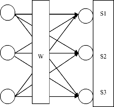
The mixing environment can be easily understood mathematically; suppose there are ‘n’ number of audio sources Si(t), i=1,2......n; and sources are equally spaced and placed in a closed recording room. All signals are captured by ‘m’ number of equally spaced microphone sensor array with transfer function hj(t), j=1,2........m; So, there are three mixing conditions. If size of source array is less than size of sensor array, then recording condition is “over determined”. If size of source array is larger than sensor array, then mixing is “under determined” and if source array and sensor array having same order then mixing is “critically determined”, which is most obvious assumption for algorithmic validation. A simple mixing model is shown in figure 1, which depicts critically determined mixing for three sources.

Independence and non-Gaussianity can be measured based on the theoretic criterion related to information, as mutual information minimization or kurtosis, a higher order static value.

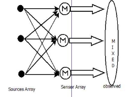
Fig.1. Mixing Model for critically determined condition

In addition, to estimate the demixing matrix by ICA methods, the metrics of negentropy, kurtosis, likelihood function, and mutual information minimization were developed [12]. Complex entropy bound minimization [13], kurtosis maximization [14], and nonlinear function based algorithms [15] takes non-Gaussianity and noncircularity into account for optimized estimation of demixing matrix. Estimation of difference between joint entropy and marginal entropy of different information sources leads to ICA implementation using minimum mutual information (MMI). Comon [16] proposed a truncated polynomial expansion to approximate the output of marginal probability density function. Hyvarinen [17] introduced a new family of contrast function for ICA using entropy approximation of maximum differential entropy. Mutual information minimization can be achieved by controlling the entropy lower bounds [15].

This work presents a modified version of convex diverge measure for optimizing the convergence speed and separation quality of existing ICA algorithms for audio source separation in blind scenario. An analysis of separated signals in case of super-Gaussian and subGaussian mixing environment is also presented and in final stage an unsupervised learning based neural architecture is proposed for weight updation in C-ICA method. The rest of this paper is organized as follows; Section II reviews importance of divergence measures and introduced modified divergence measure. Section III consist of unsupervised learning based proposed neural architecture and algorithm for weight estimation of demixing matrix Section IV comprises the analysis of separated signals in sub and super Gaussian mixing environment and an analysis of convergence speed of various divergence based ICA. Section V is collection of all simulation results based on modified convex divergence ICA and existing methods, finally conclusions are drawn in section VI.

• II.    Review of Divergence Measures

Convergence speed optimization is a key challenge in blind source separation using ICA algorithms and divergence measure implementation in weight updation equation leads to optimization of convergence speed. Amari [18] proposed the divergence method incorporating a controlling factor α and also termed as α-divergence (α-Div), which can be implemented as a measure of dependence, expressed as;

D(x, y, a ) = ——-  [1— ^ p(x, y) +

1 - a ²       2

^ p ( x ) p ( y ) - p(x,y )^{(1 -} ^( p ( x ) p(у )) ' ^{1 -} ^ХЫу

Here p(x,y) is notation for joint distribution and p(x) ,p(y) represents marginal distribution. If controlling factor substituted as ‘-1’, then Amari-Divergence turns in specialized Kullback - Liebler divergence (KL-Div), which is defined by using the Shanon entropy function H[.] [20].

DKL (x, У ) = H[p(x)] + H[p(У)] - H[p(x, У)]

= JJ P ( x , У )log

p ( x , y ) _dxdy p ( x ) p ( y )

Here DKL(x,y) > = 0 with equality if and only if ‘x’ and ‘y’ are independent to each other. By introducing joint probabilities and marginal probabilities into Cauchy-Schwartz inequality and Euclidean distance divergence can be derived, expressions are as follows;

D CS ^{( x} , У ) = log

JJ p (x, У )2 dxdy .JJ p (x )2 p (У )2 dxdy [JJ p(x, У) p(x) p(У) dxdУ]2

>

DE(x, У) = JJ(P(x, У) - P(x)P(У)) dxdy

These quadratic divergences are also reasonable to implement the ICA for Blind separation. In similar fashion,  as D ( x , y ) >  0   and Dcs(x, y ) >  0

holds true if and only if x and y are mutually independent. In Amari [18] divergence parameter α was used to optimize the convergence speed of ICA by controlling the convexity of divergence factor. Also, an f-divergence (f-Div) [19] proposed that can also be adopted as a divergence measure, can be expressed as;

D_$ ^{( x} , У ) = f f p ^{( x} ) p ⁽ У ) f I ^{P (} x ^{, У} ), '\l^dУУ

I p ( x ) p ( у ) J

Where function f(.) represents a convex function satisfying f(n)>= o for n > 0, f(n)=0 for n=1 and first order derivative with respect to n is also zero. Amari- divergence is a specific case of f-Div when, the function is defined as;

f ( n ) =

1 - a a

1 - a 1 + a      (1+a+     n - n 22

Equation (6) can be incorporated with α-Div, that measure will be equal to zero if and only if x and y are independent to each other, Zang[20].

To generalize the divergence measures Chien [21] proposed a new divergence measure based on Jensen’s inequality and Shanon’s entropy and uses it a contrast function to optimize ICA and NMF models. Convex divergence ICA (C-ICA) model constructed by incorporating joint and marginal probability into convex function with a combinational weight 0 <  X <  1 yields;

f(XP (x, y) + (1 - X) p ( x) p (y)

< Xf ( p (x, y )) +(1 - X) f ( p (x) p ( y ))

In this a work a modified version of convex function and controlled combinational weight is proposed to enhance the convexity and convergence speed. Function is expressed as;

Other values of λ. For α= 1 and -1 new NC-Div mimics C-Div but for general values of α it shows more controlled behavior. Controlled value of λ leads to control over weight distribution between joint and marginal probabilities. The convex combination is analogous to performing weighted average and creating a convex hull. To avoid undefined form of expression l’ Hospital rule can be applied by differentiating numerator and denominator with respect to α. Which gives a convex logarithmic divergence for C-Div and same expression exist for NC-Div for α= 1, -1, to achieve that simplified function first λ needs to be substituted as ½ and the l-h rule is applied but here controllability gets compromised. A comparison table is given for various divergence measures in table.1.

The comparative relation between KL-Div, E-Div, CS-Div, Amari-Div, C-Div and proposed NC-Div are described in next section. The value of convexity constant α taken between -1 to 1. For the sake of generality, a simple case of two variables (x,y) are considered in the occurrence of binary events (a,b). The marginal probabilities are Px(a), Px(b), Py(a) and Py(b) and the joint probabilities are Pxy(a,a), Pxy(a,b), Pxy(b,a), and Pxy(b,b). Above mentioned divergence measures are calculated by considering the fix marginal probability as (Px(a)=0.4 and Px(b)=0.6) , The joint probabilities Pxy(a,a) and Pxy(b,a) are set free between (0:0.4) and (0:0.6) respectively.

.^{f ( n} ) =

a

1 - a 2

1 + a 1 - a       ^{(1 -a} )X

+      n - n '2

X =

a

1 + a2

A new convex divergence (NC-Div) can be develop by incorporating equation (8), yielded as;

^{{ X} f ⁽ p ^{( x} , y )) ^{+ (1 - X ) f (} p ^{( x} ) p ⁽ y )) ^- NC , y ,      • f ( X p ( x , y ) + (1 - X ) p ( x ) p ( y ))} dxdy

=tf{ra +(1a4 ’ [1

a

1 - a a

{

1 + a 1 - a

2

2

1 - a

22

1 - a

p (x, y)- (p (x, y ))

p(x) p(y)- (p(x) p(y) /2

1 + a 1 - a

--1--

p ^{( x} , y ) ⁺

1 - a + a         )

——— p ( ^x ) p ( y ) I 1 + a ²

-

_ a             1 - a + a2           _1-a/

[----- p(x, y) + —---— p(x)p(y)] /2}}dxdy

1 + a2           1 + a2

Notably, if α considered as +1 or -1, it will result λ=1/2 from equation (8), then the joint distribution and product of marginal is permutable. This symmetric property doesn’t fit for KL-Div, f-Div, α-Div, also do not exist for C-Div and NC-Div for

0.09

0.08

0.06

0.05

0.04

0.03

0.02

0.01

0.07

0    0.05   0.1    0.15   0.2    0.25   0.3   0.35   0.4   0.45   0.5

Pxy(a,a)

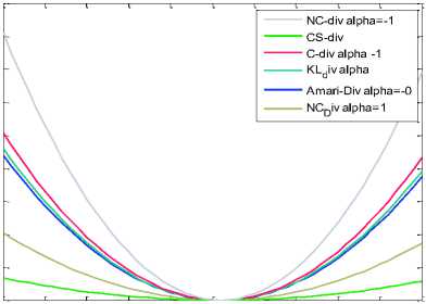
Fig.2. Behaviour of divergence Measures

0.06

0.05

0.01

0.04

0.03

0.02

0    0.05   0.1    0.15   0.2   0.25   0.3   0.35   0.4   0.45   0.5

Px,y(a,a)

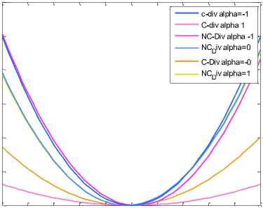
Fig.3. C-Div and NC-Div with different α

Figure 2 shows behaviour of different divergence measures by fixing the case Py(a) = Py(b) = 0.5 and graph is drawn between divergence measure verses joint probability Pxy(b,b). Divergence measures are reaching minima at same point. Figure 3 displays Amari-Div, C-ICA for α=-1 and NC-ICA for α=0, 1, -1 and result reflects that α = -1 is favourable condition for better result. Simulation result reflects that NC-Div having more convexity for α = -1 in comparison of C-Div and convexity is reducing with increment in convexity parameter.

Table 1. Behavior of divergence measure

DIV	Symmetric Divergence	Convexity	Combinational Weight	Realization from other Div
KL-Div	No	No	No	Αmari-Div (α=1)
Αmari-Div	No	α	No	f-Div (conditional function)
f-Div	NO	α	No	No
JS-Div	λ=1/2	No	λ (Convex)	C-Div (α=1,λ=.5) NC-Div (α=1)
Convex log Div	λ=1/2	No	λ (Convex)	C-Div(α=1,λ=.5), NC-Div (α=1)
C-Div	λ=1/2	α	λ (Convex)	By (8)
NC-Div	λ=1/2 or α=+/-1	α	λ (Convex)	C-Div (α=1 &-1)

Different divergence measures (defined in previous sections) can be incorporated in “10” and various ICA procedure based on divergence measures can be develop. However in the natural gradient learning method, the KL-ICA experiences from the problem of divergence of convergence to matrix with certain scaling shift if weight is not initialized properly. Experiment is performed by taking fix threshold value and an audio signal of 3sec taken from the Ghost Buster movie, one male voice sample of same duration and one female voice sample of equal duration. And the comparative results of various divergences based ICA is shown in figure 4. In this graph NC-ICA stabilized between 80 to 100 epochs and C-ICA stabilized after 100 epochs which depicts NC-ICA converges 20% faster than C-ICA.

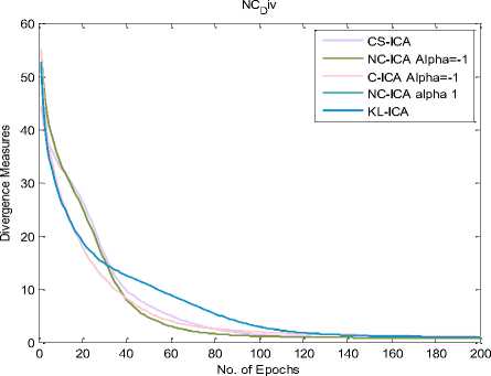
Fig.4. Learning curves of various divergence based ICA algorithms for (alpha 0,1, -1)

• III.    Unsupervised Learning

In unsupervised learning process for the training input vector, when the target output is not known. The neural network may modify the connecting weights so that the most similar input vector is assigned same group of output. Unsupervised networks are more complex and difficult to implement.

X1

X2

X3

Weight Matrix     Separated Data Output

Mixed Data Input

Fig.5. Neural Structure for Blind Audio Source Separation

For an unsupervised learning rule, the training set consists of input training patterns only. Therefore, the network is trained without benefit of any teacher. The network learns to adapt based on the experiences collected through the previous training patterns. The blind audio source separation problem can be correlated to unsupervised learning, as in this problem the intention is to estimate demixing matrix which can nullify the effect of mixing matrix and neural structure to short out this problem can be proposed as in figure 3.

In proposed neural architecture proposed in figure 5 X=[X1 X2 X3] is a mixed version of audio signals, to unmixed signals the weight are stored in W matrix and a learning algorithm is applied which is based on modified convex divergence measure proposed in section II “(9)”. The complete algorithms is as follows

Step 1.      Load mixed signal matrix ‘X’

Step 2.     Perform Mean removal (Cantering)

X ^ X-E[X]

Step 3.      Whitening of X using eigenvalue and

Eigenmatrix

X ^ ф D-1/2фT X ; Here ф and D denotes eigenmatrix and eigenvalue of matrix E[XXT]

Step 4.      Define Learning rate

No of iterations required α(alpha) = -1, 1, or .5 (Here we assumed -0.99)

Time start and time finish (As per input signal)

Step 5.      Initialize weight matrix

W ^ Rand(m,n)

Step 6.      Perform Centering over W as in step 2;

W ^ W-E[W]

Step 7.      Repeat step 8 and 9 for K= 1: No of

Iterations

Step 8.      Update weight using scaled natural

Gradient methods as in equation

_W ( t + 1) _{= W} ( t ) _{- η} ^{c   ∂ D}NC ^{( χ , W  , α )} _W ( t ) T _W ( t )

_d ( t )         _{∂ W} ( t )

Here; DNC(X,W,α) defined in “(9)”, η learning rate, ‘c’ and ‘d’ are used to stabilize the learning rate explained in [21].

Step 9.     Normalize the W as W ^ W/||W||

Step 10.    Esti_W ^ W+ n* W

Step 11.    W ^ Esti_W* Whiten_matrix

Step 12.    W ^ W+E[W]

Step 13.    Demix signals S ^ X*W

Step 14.     Check fixed positive Kurtosis Values as

Defined in [14] for each signal (reason Explained in section IV)

Step 15.     If up to desired value go to step 13 else go to step 5

Step 16.     Evaluated The quality of separation using

BSS Eval function

BSS_Eval(Estimated, Desired) BSS_Eval function described in [11]. Available under GNU public license.

There are certain important point to note during implementation of proposed algorithm, as data preprocessing and post-processing is very essential, that includes whitening and centering process. Second key point of concern is weight initialization; the motivation of weight initialization is taken from fast-ICA but in this algorithm method of weight updation in improved and more efficient. Another important point is fixing the threshold value to execute the weight updation mechanism and ensuring the quality of separation. To derive a generalized concept for threshold value and experiment has been performed over sub-Gaussian and super-Gaussian mixing environment, explained in section IV. Which advocates a positive kurtosis value should be taken for ensuring good quality of separation, as result suggest in following section; that nature of separated signal component is always super-Gaussian in nature.

• IV.    Signal Separation in sub and Super-Gaussion Mixing Environment

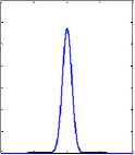
According to central limit theorem the PDF(Probability Distribution Function) of mixed Non-Gaussian source signals is Gaussian in nature. A linear combination of number of independent signals is called a Gaussian signal. Separating the independent sources from a Gaussian signal is carried by transforming the signal into nonGaussian signal. Non Gaussian signals are The Probability Distribution Functions of super-Gaussian and sub-Gaussian signals are shown in the figure 6 and figure 7 respectively.

The broken lines in the Figure 6 and Figure 7 plot the distribution of Gaussian nature of signals. From the Figure 6 it is clear that the peak of the distribution of a super-Gaussian signal is higher than that of a Gaussian signal. While in Figure 7 it is evident that the subGaussian signals have a spread distribution.

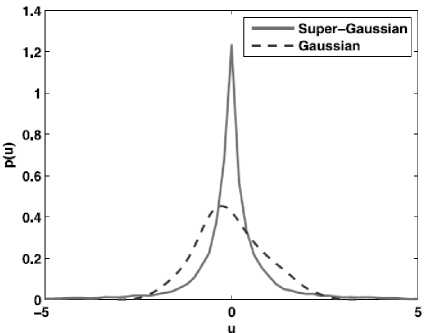
Fig.6. Super-Gaussian signals [11]

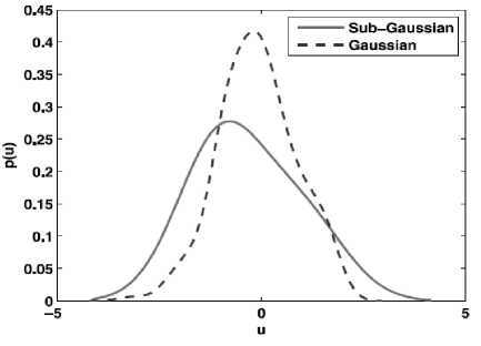
Fig.7. Sub-Gaussian Signal [11]

Evaluation of the quality of separation in case of subGaussian and super-Gaussian mixture environment performed as follows

Three signal’s were taken and mixed by a random sub and super-Gaussian mixing environment and signals were separated by sub-Gaussian and super-Gaussian ICA approaches and resultant sub and super-Gaussian probability distribution function of separated signal are shown is Figure 8 and 9 respectively. Results presented in Figure 8 and Figure 9 having positive kurtosis value of independent components for separated signals in subGaussian and super-Gaussian mixing environment both, which clearly indicates that separated signals are always super-Gaussian and does not depends on mixing environment. Hence for proper implementation of algorithm presented in previous section positive kurtosis value can be used as threshold parameter on separated components for weight updation.

• V.    Simulation and Result Discussion

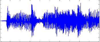
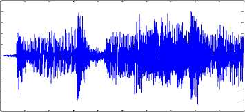
  To evaluate the performance of proposed algorithm is section III an experiment has been performed. In this experiment three signals have been taken and 20000 samples have been loaded of each signal. To evaluate quality of separation three audio recordings has been taken; one recording ‘Tabla’ a traditional Indian musical instrument, one drum beat recording sample and one car horn sample. Previous to samples are recorded in a closed glass chamber to maintain idea mixing environment, where no noise component is taken into account. Signals were mixed using a randomly generated a 3X3 matrix. Mixed signals are normalized by dividing by the standard deviation of mixed signals. Mixed signals are shown in figure 10 (a), 10(b), and 10(c). This reflects that in mixture 1 signal 3 is dominant and signal 1 and signal 2 are dominant in mixture 2 and mixture 3.

In addition to perform and instantaneous BASS task, we evaluated different ICA methods. The primary task targeted to separate signals from mixture with assumption there is no noise contamination, i.e. X= AS. The second objective is to evaluate separation performance of algorithms, in terms of signal to interference ratio.

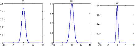
Fig.8. Independent components Kurtosis value for Super-Gaussian mixing

-5

mixed signal 2

-1

-2

-3

-4

0.2

0.4

0.6

0.8

1.2

1.4

1.6

1.8

2 x 104

Fig.10.(b). Mixed Signal 2

S'1

-10      -5       0       5      10

0.7

0.6

0.5

0.4

0.3

0.2

0.1

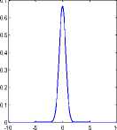
Fig.9. Independent components Kurtosis value for Sub-Gaussian mixing

mixed signal 3

-1

-2

-3

-4

0.2

0.4

0.6

0.8

1.2

1.4

1.6

1.8

2 x 104

Fig.10.(c). Mixed Signal 3

In implementation of proposed algorithm the sub and super-Gaussian mixing environment is not a matter of concern and positive kurtosis threshold is valid in general.

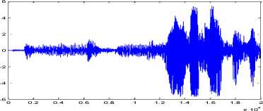
Fig.10.(a). Mixed Signal 1

For validation of algorithm proposed in this paper, the mixture of signals were separated by using JADE, Fast-ICA and C-ICA for alpha=-1; and results were compared by separated signals using proposed NC-ICA alpha=-1.

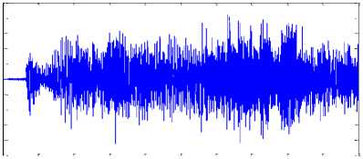
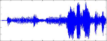
During implementation of proposed algorithm weight initialized using method suggested in section III and after estimation of demixing matrix, demixing matrix multiplied with mixed signals and again mean value added to separated signals in post-processing to neutralize the effect of centering process. Separated signals are shown in figure 11(a), 11(b) and 11(c).

-5

demix signal 1

-1

-2

-3

-4

0.2

0.4

0.6

0.8

1.2

1.4

1.6

1.8

2 x 104

Fig.11.(a). De-mixed Signal 1

demixed signal 2

-1

-2

-3

-4

algorithms like JADE, Fast-ICA, C-ICA and proposed algorithm NC-ICA. The quality of separation is good for signal 2 and there is a significant difference between performance of proposed ICA and other competitor. On the other hand for signal 1 and signal 2 SIR values obtained by NC-ICA is significantly better than JADE and Fast-ICA but there is mild advantage over C-ICA. Figure 11 suggests that, signal strength is better in signal 2 and comparatively weak in signal 1 and signal 3. Which could be a reason behind minor difference between performance of algorithms with same convexity parameter ‘-1’. But it also reflects if signal strength is good in any mixing environment, then proposed algorithm is better performer than existing convex divergence ICA for same convexity parameter.

Figure 12 shows comparative analysis of separation quality by various ICA algorithms and proposed algorithms. Algorithms have been applied over same mixture and result suggests that NC-ICA gives good separation quality in terms of signal to interference ratio in dB. Proposed algorithm NC-ICA gives in an average 6-7% better result than C-ICA, 12-16% better result than Fast-ICA and 20-24% better than JADE algorithms. In section III it has been proven that the convergence speed of proposed NC-ICA algorithm is better than existing algorithms. The conclusion can be drawn from this analysis that proposed algorithm gives better result in terms of convergence speed and separation quality. So, it can be adapted as a better Blind Audio Source Separation Technique.

-5

0.2

0.4

0.6

0.8

1.2

1.4

1.6

1.8

4 x 104

-6 0

Fig.11.(b). De-mixed Signal 2

demixed Signal 3

-2

-4

0.2

0.4

0.6

0.8

1.2

1.4

1.6

1.8

2 x 104

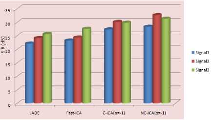
Fig.12. Separation Quality Comparisons

Fig.11.(c). De-mixed Signal 3

The Quality of separation of separated signals by each algorithm is evaluated by Bss_Eval function available under GNU public license for Matlab framework. A comparative analysis is given in Table 2.

Table 2. Separation quality of JADE, Fast-ICA, C-ICA and NC-ICA

SIR(dB)/ Algorithm	JADE	Fast-ICA	C-ICA (а=-1)	NC-ICA (а=-1)
Signal1	22.10	23.20	27.30	27.80
Signal2	24.10	24.30	30.10	32.20
Signal3	25.60	27.50	29.80	30.30

The performance of ICA algorithms is determined by quality of separation and for the same objective signal to interference ratio is evaluated. Table 2 consist of SIR value in dB for signal 1, signal 2 and signal 3 against

In this analysis effect of noise component is not taken into consideration, if there is noise contamination in mixed signal. Then mixing model can be represented as; X= A.S+ n, which degrades the quality of separation and complexity of algorithms increases as well. As noise removal before execution of weight estimation algorithms becomes a necessity. In this paper ideal mixing environment is considered but this work can be further extended for noise contaminated mixed signal.

• VI.    Conclusion

ICA Algorithms are chosen as a better option for audio source separation in blind scenario. There are certain challenges in implementation of ICA algorithm for BASS. As convergence speed gets compromised when quality of separation is taken into account. Divergence based ICAs are emerging options. Proposed ICA algorithm is based on optimization of unsupervised learning based weight estimation technique. Learning equation derived based on divergence measure having controlling convexity parameter and scaled natural gradient method is included in learning process. In proposed algorithm weight initialization technique is included to enhance convergence speed along with quality of separation. The important findings of this research are, Separated signals are always super-Gaussian irrespective to mixing environment and separation technique; Proposed algorithms convergence speed is 20% faster than existing algorithm for same convexity parameter and gives better separation quality in comparison of existing ICA techniques as Fast-ICA and JADE. In this work ideal mixing condition is taken but this work can be further extended for source separation in noisy mixing environment.

• [1]    Sebastian Ewert, Bryan Pardo, Meinard Muller and Mark D. Plumby, "Score-Informed Source Separation for Musical Audio Recordings", IEEE Signal Processing Magazine, May 2014, pp. 116-124

• [2]    P. Comon and C. Jutten, Handbook of Blind Source Separation; Independent Component Analysis and Applications, 1^st ed., New York, USA: Academic, 2010.

• [3]  A. Hyvarinen, J. Karhunen, and E. Oja, "Independent

  Component Analysis".New York: Wiley, 2001.

• [4]    G R Naik and Dinesh K Kumar, "An Overview of Independent Component Analysis and Its Applications", Informatica (35), pp. 63-81, 2011.

• [5]    Hansen, "Blind Separation of noisy image mixtures", Springer-Verlag, pp. 159-169, 2000.

• [6]    D.J.C Mackay, "Maximum likelihood and covariant algorithms for independent component analysis", University of Cambridge London,Tech.Report,1996

• [7]    H. Attias and C. E. Schreiner, "Blind Source Separation and deconvolution: The dynamic component analysis algorithm," Neural Computing, Vol. 10, No. 6, pp. 13731424, August 1998.

• [8]    M. S Lewicki and T. J. Sejnowski, "Learning overcomplete representations," Neural Computing, Vol.12, No.02, pp. 337-365, February 2000.

• [9]    A. Hyvarinen, R. Cristescu, and E. Oja, "A fast algorithm for estimating overcomplete ICA bases for image window", Neural Networks, Vol.02, pp.894-899, 1999.

• [10]    A. Hyvarinen, J. Karhunen, and E.Oja, "Independent Component Analysis", Wiley-Interscience, May2001

• [11]    Geng-Shen Fu, Ronald Phlypo, Matthew Anderson, and Tülay Adali, "Complex Independent Component Analysis Using Three Types of Diversity: Non-Gaussianity, Nonwhiteness, and Non-circularity", IEEE Transactions on Signal Processing, Vol. 63, No. 3,pp.794-805, February 2015

• [12]    P. Comon, “Independent component analysis, a new concept?,” Signal Process., vol. 36, no. 3, pp. 287–314, 1994.

• [13]    Y. Chen, “Blind separation using convex function,”IEEE Trans. Signal Process., Vol. 53, No. 6, pp. 2027–2035, Jun. 2005.

• [14]    H.Li and T. Adali, “A Class of complex ICA algorithms based on the kurtosis cost function”, IEEE Transaction Neural Networks, Vol. 19, No. 3, pp. 408-420, Mar. 2008.

• [15]    X-L Li and T. Adali, “Complex independent component analysis by entropy bound minimization,” IEEE Trans. Circuits Systems, Reg. Paper, Vol. 57, No. 7, pp. 14171430, Jul 2010.

• [16]    P. Comon, “Independent component analysis, a new concept?,” Signal Process., vol. 36, no. 3, pp. 287–314, 1994.

• [17]    A Hyvarinen “Fast and robust fixed point algorithms for independent component analysis”, IEEE Transactions on Neural Networks, Vol.10, No.3, pp.626-634, 1999.

• [18]    Amari, “Natural gradient works efficiently in learning,” Neural Computing Vol. 10, pp. 251–276, 1998.

• [19]    Csiszár and P. C. Shields, “Information theory and statistics: A tutorial,” Foundations Trends Commun. Inf. Theory Vol. 1, No. 4, pp. 417–528, 2004.

• [20]    Zhang, “Divergence function, duality, and convex analysis,” Neural Computing., Vol. 16, pp. 159–195, 2004.

• [21]    Jen-Tzung Chien and Hsin-Lung Hsieh, “Convex Divergence ICA for Blind Source Separation”, IEEE Trans. Audio, Speech, and Language Processing, Vol. 20, No. 01, pp. 302-314, January, 2012.

• [22]    Sugreev Kaur and Rajesh Mehra, “High Speed and Area Efficient 2D DWT Processor Based Image Compression”, Signal & Image Processing : An International Journal (SIPIJ) Vol.1, No.2, pp. 22-30, December 2010

• [23]    S. C. Douglas and M. Gupta, “Scaled natural gradient algorithms for instantaneous and convolutive blind source separation,” in Proc. Int. Conf. Acoust., Speech, Signal Process., pp. 637–640, 2007.