A Hybrid Deep Learning Ensemble with Wavelet Feature Extraction for Stock Market Prediction

Investment, capital formation and economic development is possible only in the stock market, the backbone of the modern economy. The prices of stock, however, are highly volatile and depend on numerous factors, including macroeconomic factors, politics, market sentiment and investment psychology. Such complexities result in extreme difficulties to clearly foresee future outcomes of decisions but reduced risk levels require investment and finance assumptions and choice-making deliberations by the investors, financial institutions, and policies [1]. Some of the traditional model statistics that have largely been used when it comes to predicting finance are ARIMA and regression model. Stationery behavior and assumptions however do not include the explicit destabilization of motions and chaos of the financial information [2].

With the emergence of machine and deep learning, its capacity to unearth the pattern of data not evident in significant volumes and noises is truly amazing [3]. Some of the most popular sequence learning models, which have been effectively applied to discover temporary correlations in the financial time series are the recurrent deep net known as the recurrent nervous network (RNN), long short-term memories (LSTM), and gated recurrent unit (GRU) [4,5]. Convolutional Neural

This work is open access and licensed under the Creative Commons CC BY 4.0 License.

Networks (CNNs), originally created as a computer vision model, have additionally been used to forecast finances, where they are proving efficient at eliminating local patterns and short-term features [6]. Despite this, all of the above standalone models were discovered to have some weaknesses even in the absence of considering training and evaluation cards: RNNs cannot learn long-term dependencies due to vanishing gradients, LSTMs can operate well only on large datasets and with significant computation analysis capabilities, GRUs are efficient networks, but due to the lack of detailed dependency features owing to the nature of their encoded features, and CNNs fail to model sequential dynamics explicitly [7].

Among strategies to overcome these limitations, increasingly researchers address such strategies as hybrid and ensemble. Combination of wavelet transform, stacked auto-encoders and LSTM is indeed effective to predict financial time series. Moreover, recent works have proposed more such hybrids such as Capsule Network which is LSTM structures, wavelet-ARIMA-LSTM and Transformer based hybrids with attention structures to predict at high frequency. These practices enhance the upward trend of recreational profits of the model supplement to generate strength and accuracy. Signal decomposition has similarly experienced another important development in parallel with the idea of hybridization. Specifically, the Discrete Wavelet Transform (DWT) has emerged as one of the most efficient financial forecasting methods, as it decomposes the noisy stock time series into different levels of resolution and eliminates the high-frequency variation without losing the time and frequency techniques [8,9,10]. More recently, new ideas like WEITS (Wavelet Enhanced Interpretable Time Series) or other wavelet-pre-processing systems have also attested to the robustness of decomposition on multi-scale in stock prediction task [11].

Although these studies have advanced the state of the art, most of the existing methodologies are constrained. The majority of them are based on a combination of only two architectures, whereas some are based on one paradigm, like Transformers or Capsule Networks. Not many works have been attempting to fuse a couple of complementary deep learnings along with a wavelet based pre-processing. The existence of such a gap motivates the present study that proposes a novel ensemble deep learning structure with DWT to enhance the strength and extrapolation of stock prices. It uses the RNN, LSTM, GRU, CNN structures and differentiates local and short time features, sequential dynamics as represented by RNN, long time dependencies represented by LSTM and GRU and finally separates input data into multi resolution subcomponents to eliminate noise and preserve trend information.

There are three major contributions of this research. First, it introduces a DWT integrated ensemble that simultaneously performs four deep learning architectures offering a broader synergy than any tested models before. Second, it makes comparisons of the framework with six real world databank (NIFTY 50, BRITANNIA, HDFCBANK, RELIANCE, TataSteel and TITAN) and in all cases the framework performs better than the individual models on accuracy and reduced error measures. Third, it reveals that the framework has potential whenever a decision support system to which investors can turn to make sound and interpretable predictions in the face of volatile markets. It offers a computationally feasible hybrid framework to the financial forecasting field and extends the limits of deep learning applications to the stock market by combining ensemble learning with wavelet based pre-processing.

Stock market forecasting is an actively studied field over the last few decades, but the paradigm of the task has been evolving as more conventional statistical models are replaced by increasingly complex machine learning and deep learning technologies. The corresponding works are analyzed in this section in three dimensions, that is, in the theories of classical statistics, deep learning networks, and deep learning model with wavelet-based preprocessing, and in ensemble/hybrid model. The initial works were mainly statistical and econometric model ARIMA, GARCH and regressions. However, despite obtaining decoding findings and being useful in non-portable states, these approaches could not reflect a dynamic dependence on nonlinear fluctuations in stock prices [12]. Since the introduction of deep learning, LSTM and Gated Recurrent Units (GRU) models have become reasonable across time-series prediction along with Recurrent Neural Networks (RNNs). The vanishing gradients and training long-term dependencies were specifically considered with the LSTM networks, and provided the GRUs were a computationally efficient source. The financial forecasting models of CNNs were next trained to learn local time-dependence and high-frequency fluctuations. Though these independent models were observed to be powerful, sensitive to noise, overfit and they were also insensitive to multiscale features [13].

The number of studies dealing with hybrid and ensemble models did increase in an attempt to overcome these limitations. The first time combined wavelet transform with stacked auto-encoder/LSTM and showed that decomposed features lead to significant improvement of prediction quality. Some more recent results include CNN-LSTM ensembles, Capsule Network LSTM models, Transformers-based ensembles, etc. Whilst these frameworks make use of the complementarity between different architectures, they are often specific to two-model combinations or computationally expensive [14].

With the growing architecture, wavelet-based pre-process has become yet another enabling technology for financial forecasting. For stock data, it has been used for de-noising of stock signals and extraction of features at different scales respectively which makes the subsequent model more robust. Machine learning models to detect the NIFTY 50 index and found that the pre-processing of wavelets was indeed a big help. Wavelet-Enhanced Interpretable Time Series (WEITS) or wavelet-ARIMA-LSTM hybrids suggest multi-scale decomposition is on the verge of producing very powerful and interpretable prediction solutions [15]. However, in Table 1 states studies combining wavelet architectures and a single deep learning model mostly focused on fitting the wavelet to a single deep neural network, or linear models that do not deal with the issue of multi-architecture wavelet-adapted ensembles.

Table 1. Summary of related works

Author & Year	Method / Model	Dataset	Key Findings
Meesad et al. (2013)	Support Vector Regression	Stock price index	Provided better accuracy than linear regression
Jia (2016)	LSTM	Stock price time series	Captured long-term dependencies effectively
Hiransha et al. (2018)	LSTM, RNN, GRU	NSE stock market	GRU outperformed RNN, LSTM in speed and accuracy
Hoseinzade et al. (2018)	CNN (CNNPred)	S&P 500, DJIA	CNN captured local temporal dependencies
Bao et al. (2017)	Stacked Autoencoder + LSTM + Wavelet	Shanghai Stock Exchange	Wavelet pre-processing improved prediction
Nagula et al. (2022)	ML approaches (RF, SVM, ANN)	NIFTY 50 index	Gave competitive short-term predictions
Zhou et al. (2022)	CNN-LSTM hybrid	CSI 300 index	Combined CNN feature extraction with LSTM memory
Arif et al. (2023)	1D CapsNet + LSTM	S&P 500	Captured hierarchical features and temporal patterns
Jarrah & Salim (2019)	RNN + DWT	Stock price index	Wavelet decomposition reduced noise effectively
Fathali et al. (2022)	ML models + DWT	NIFTY 50 index	Improved predictive accuracy using wavelets
Zhang et al. (2024)	Hybrid Wavelet–ARIMA–LSTM	Stock index futures	Multi-resolution features improved forecasts
Wang et al. (2024)	WEITS (Wavelet-Enhanced Interpretable Time Series)	Financial & energy datasets	Wavelet + residual framework improved interpretability
Zhang et al. (2025)	HAELT: Hybrid Attentive Ensemble Transformer	High-frequency stock data	Outperformed baselines with ensemble attention

In general, three major gaps in literature are identified. The standalone models, although quite powerful, are not sufficient enough to deal with the complexity of noisy nonlinear financial information. Second, the current hybrid models only take two architectures into account, which does not allow taking advantage of the wider model complementary. Third, wavelet pre-processing has proved to be a very promising method, but its implementation into multi-model ensemble models has not been well-explored. These doom gaps encourage the current study, which suggests a new DWT-based ensemble of RNN, LSTM, GRU, and CNN architectures, with an aim of integrating time-based, nonlinear, and frequency based representations into the single framework to make the stock market forecasting robust.

3.    Methodology

The multi-stage pipeline has been used in the proposed methodology to determine precise forecasts of the stock market. Stock market data is highly hectic, unclear and affected by short-time volatility and long term trend. To overcome these issues, the framework combines pre-processing, wavelet-based feature extraction, and a collection of deep learning models (RNN, LSTM, GRU, and CNN), each being specific to the characteristics of financial time series. As opposed to traditional single model methods, the ensemble enjoys the benefits of complementary design-RNNs to capture sequential dependencies, LSTMs to capture long-term memory, GRUs to capture computational efficiency, and CNNs to capture short-term pattern recognition. The combination of these architectures on wavelet-decomposed features in the methodology yields robustness to market noise as well as adaptation to a variety of stocks. This means that it is highly predictive and directionally reliable, suitable in the real-life trading and investment decision support.

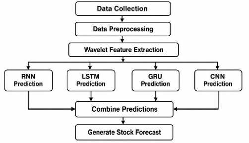
Fig.1. Flowchart of the proposed methodology

The full workflow of the proposed model is presented in a sequential fashion in the Algorithm 1. It starts with the stock market data being acquired and prepared whereby any missing elements are interpolated, abnormal stock market data corrected and the series then normalized. In order to map the information into a supervised learning format, a fixed sliding window is used whereby past observations can be mapped into future-based predictions. Normalized sequences are then converted using the Discrete Wavelet Transform (DWT) which splits the signal into approximation (trend related) and detail (fluctuation related) parts. The input of these decomposed features is presented to four different deep learning networks- RNN, LSTM, GRU and CNN- each network is set to identify various temporal or structural variations of stock price movements. Finally, an ensemble fusion mechanism combines the model predictions using weighted averaging to generate the next-day closing price forecast.

Algorithm 1: Proposed Hybrid Ensemble Framework

Step 1: Collect OHLCV data for NIFTY50, BRITANNIA, HDFC, RELIANCE, TATASTEEL, TITAN

Step 2: Extract closing price series as prediction target

Step 3: Preprocess data: (a) Handle missing values (linear interpolation), (b) Normalize using Min-Max scaling, (c) Generate supervised sequences with 30-day sliding window

Step 4: Apply Discrete Wavelet Transform (DWT): Decompose into approximation (A) and detail (D) coefficients Step 5: Train models on DWT features: RNN (short-term), LSTM (long-term), GRU (efficient), CNN (local motifs) Step 6: Ensemble Fusion: Mean aggregation of model outputs

Step 7: Evaluate model using RMSE, MAE, R2, and Directional Accuracy

Step 8: Output next-day predicted closing price yt+1.

• 3.1.    Data Collection

• 3.2.    Data Pre-processing

Six major Indian equities-NIFTY 50, Britannia, HDFC Bank, Reliance, Tata Steel and Titan stock data of the market in terms of bull run, bearish market and disruption events like the COVID-19 pandemic were gathered in the form of daily historical stock data in Yahoo Finance over ten years. The data contains OHLCV (Open, High, Low, Close, and Volume) characteristics that are common in technical and quantitative financial analysis. Of these, the closing price was selected as the target variable since it is a more accurate consensus estimate of the market at the end of the trading day, is less susceptible to intraday noise, and is the input to many technical indicators including RSI, MACD, and Bollinger Bands. The closing price also gives uniformity to the past forecasting research, which makes reproducibility and comparison of results possible [16].

A sequence of pre-processing algorithms prepares the data to be utilized to a deep learning model. The operations will reduce the level of noise, correct anomalies, and convert the raw time series into a format that will easily be learns by the models. Pre-processing steps include:

• •    Handling Missing Values: The common cause of price gaps in the historical stock data is routing issues and holidays. In terms of time series data maintenance, the gaps were filled with forward filling the gaps of missing values.

• •    Outlier Treatment: Outliers were treated using statistical thresholds in order to smooth spikes or wrongly recorded data, which would otherwise pollute the training process in the form of extreme outliers.

• •    Normalization: The prices of companies are different (e.g., Reliance ~ Rs. 2500 vs. Tata Steel ~ Rs. 120). MinMax normalization ensures comparable scales:

[^d^ ft+ll i^i^ tt+T-l} ] ⁴ ^ {t+т}                                    ⁽¹⁾

where:

• •    X = original stock price value (e.g., Reliance closing price = Rs. 2500),

• •    X min = minimum price in the dataset (e.g., Reliance’s lowest closing = Rs. 1800),

• •    X max = maximum price in the dataset (e.g., Reliance’s highest closing = Rs. 2800),

• •    X norm = normalized value, scaled between 0 and 1.

If Reliance’s price today is Rs. 2500, normalization gives:

Y     _ (2500 - 1800)

— = 0.7 1000

^Амгт = (2800 - 1800)

This makes all stocks comparable on a standard scale of 0 -1, such as Reliance at Rs. 2500 and Tata Steel at Rs. 120. Otherwise, models can give a premium to more expensive stocks. Neural networks are scale-sensitive and unless the data are normalized, the model may select titles such as Titan (Rs. 3000) than Tata Steel (Rs. 120) just because they have higher values. Normalization provides balanced and equitable learning.

• •    Sliding Window Transformation: The stock market forecasting can be considered a sequence-dependent issue, there-fore, a sliding window transformation was implemented to generate supervised learning samples. The prediction was based on a preset size look-back window (e.g., 30 days) to make the next-day price prediction:

  [ЗД_£+1} ,

  
  

  -,^ {t+T-1} ] ^ ^ {t+T}

  
  
  
  

• 3.3.    Feature Extraction with DWT

Input: A sequence of T past prices (e.g., last 30 days closing prices).

Output: The next day’s price (X { _t+1 } ).

Example: Suppose a 5-day window ( T = 5) is used.

Inputs: [ Rs. 2500 , Rs. 2520 , Rs. 2515 , Rs. 2530 , Rs. 2540] ^ Output: Rs. 2550

It is reflective of the way traders usually make a market analysis: examining the last month of price movement to predict the future. By shifting the window across the dataset, thousands of training samples are created, enabling the model to interpret historical sequences and predict future movements [17]. Even though the evaluation is being made on the basis of the close prices, the deep learning models are trained on the logarithmic returns to reduce non-stationarity and stabilize the variance. The use of log-return transformation has become very common in the financial time series and it is also used in financial analysis because the behavior is almost truly stationary. The returns that have been predicted are then converted back to price space to be evaluated in terms of performance.

Financial time series are multi-scale in nature: short timescale fluctuations (noise) and longer timescale cycles (trend). Discrete Wavelet Transform (DWT) was applied to the stock signal for approximation (trend) and detail (fluctuation) decomposition:

^(t) = T^Ajtbjtt) ⁺ ^j^Dj^jtt)                              ⁽³⁾

For instance, when using approximate coefficients to predict NIFTY 50, the quarterly NIFTY 50 momentum is captured in the approximate coefficients, while one-day shocks (such as Titan’s dip after an earnings announcement) are reflected in the detail coefficients. This de-noising improves the signal-to-noise ratio, making it possible to learn meaningful patterns without overfitting on random volatility.

• 3.4.    Wavelet De-noising and Decomposition (DWT)

The price of a stock market is non-stationary, noisy, time series of multi scales, and prone to volatility on a daily basis, macroeconomic cycles and random events. To deal with such complexities, Discrete Wavelet Transform (DWT) was applied to the decomposition and de-noising of the data and then inputted into the deep learning models. Because of the non-stationary and noisy character of the stock data, the effect of DWT as a feature extraction method was employed. Wavelet transforms, in contrast to Fourier transform, do not just yield information in the frequency domain, but offer time frequency localization, so that they are particularly effective on financial time series with both short-term and long-term variations.

Mother wavelet that was applied in this work was Daubechies-4 (db4) mother and the level of decomposition was two. The reason why db4 wavelet was selected is that its support and smooth nature are small enough, and thus suitable in the analysis of financial time series that show sharp oscillations and slow gradual movements. In order to achieve a trade-off between noise reduction and maintenance of meaningful temporal structures, a moderate level of decomposition was selected, localization it offers, which is appropriate in financial time series that has both sharp and smooth changes. DWT is computationally efficient and offers deterministic multi-resolution analysis to daily stock data as compared to other empirical methods of decomposition like EMD or VMD [17]. DWT breaks down the original time series into:

• •    Approximation coefficients (low-frequency) – capturing long-term trends.

• •    Detail coefficients (high-frequency) – capturing short-term volatility and noise.

This decomposition helps to focus the models onto relevant multi-scale patterns and isolate the noise, ultimately leading to stronger and more accurate predictions. DWT can also be used as a signal processing analyzer to analyze time series x(t) as to approximation and detail coefficients at various scales (that is why it is also known as multi-resolution analysis). The decomposition can be expressed as:

x(t) = E^ a_jo^(_{i o} ,_k)tt) + У^₀ У .    d^^tt)                    (4)

Where:

• •    ^a j₀, _k: Approximation coefficients (low-frequency trends)

• •    d j, _k: Detail coefficients (high-frequency components)

• •     Ф (1оЛ) ( t ): Scaling functions

• •    ФикЖ t ): Wavelet functions

• •    j : Level of decomposition

• •    k : Translation parameter

The components of the decomposition in the DWT system play a direct role in decomposing the stock price series into important patterns at multiple time scales. The approximation coefficients (a_Jo , _k ) reflect the long-term structural changes i.e. gradual increasing or decreasing movements as a result of macroeconomic conditions or quarterly performance. The detail coefficients (d j, _k ) on the other hand, represent the volatility in the short term due to unforeseen news, investor responses or market microstructure noise. The area of scaling functions ( Фа₀, _к ) ( t )) are approximations of low-frequency components, whereas the area of wavelet functions (tp (j, _k ) ( t )) are local effects of change, both in time and frequency. The order of decomposition j is denoted by the parameter and with smaller values reflecting momentary fluctuations and greater ones long-term trends. These functions are translated by the parameter k to stress on time axis, which makes it possible to reconstruct time variation. Collectively, these elements enable the creation of a multi-resolution stock price process, that is, noise at the micro-level, and trend behavior at the macro-level, resulting in cleaner and more organized inputs to deep learning models [18].

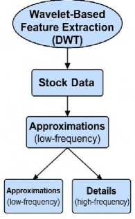
Fig.2. Wavelet decomposition process of stock price data into approximation (A) and detail (D) components

Approximation coefficients are used in the analysis of the long-run dynamics of the stock price in demarcating longterm cyclical movements, e.g., around the announcements of quarterly earnings, or an overlaying economic cycle. On the other hand, the short run volatility is represented by detail coefficients, such as sharp price changes caused by corporate announcements. As an example, the approximation and detail components in the NIFTY 50 index reflect macrolevel dynamics occurring over multiple months and high-frequency dynamics caused by daily market dynamics or one event respectively. The discrete wavelet transform provides a multi-resolution representation of an image, which contains fewer noise points and more informative, salient structural information, by selectively filtering out the noise on the detail coefficients and keeping only the salient structural elements.

The wavelet decomposition process is expounded in Fig. 2. The input signal (closing price series) is steadily flattened by low-pass filter (scaling function, ϕ ) and a high-pass filter (wavelet function, ψ ). The approximation remains contained within the low-pass component, denoted A, and, therefore, an indicator of the long-term form, and the high-pass component, which results in the detail, denoted D, which is an indicator of short-term volatility [18].

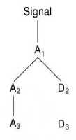
Fig.3. Multi-level wavelet decomposition tree showing hierarchical breakdown

Fig. 3 shows a multi-level decomposition tree. At each level, the approximation part is further divided into new approximation and detail coefficients. At the third level, the signal is represented as:

Signal = A 3 + D 3 + D 2 + D 1                                  (5)

This hierarchical representation demonstrates how DWT reflects both long-term stock price trends (deepest approximation) and short-term volatility (detail coefficients). The multi-resolution representation clarifies why DWT is suitable for de-noising and feature extraction in financial forecasting tasks. In order to overcome look-ahead bias, Discrete Wavelet Transform was used applied within each rolling training window of the walk-forward validation protocol. During each iteration, only history observations till the point of prediction were broken down so that feature extraction was not counted on future information. This time-based implementation can avoid information leak and maintain out-of-sample evaluation integrity. The wavelet decomposition and scaling were conducted on all preprocessing responses followed by chronological splitting in each training window.

• 3.5.    Deep Learning Models for Stock Prediction

Stock market data is a non-linear, dynamic, noisy system having short-term volatility while also exhibiting longterm dependencies. In order to model such complexities, we employ four complementary deep learning architectures: RNN, LSTM, GRU and CNN. All of the models examined in this paper represent a different aspect of financial time series, including high-frequency intraday sequential movement and quarterly cyclical methods and localised trade behaviour. In many cases, a TypeInfo any of models has the strength of overcoming the weaknesses of an individual model due to an integrative amalgamation of the models as has been demonstrated in comparative studies on stock-price forecasting. The production of shared wisdom is a process that can be characterized as an integrative process, hence diversifying our holistic knowledge about market dynamics–a strategy supported in recent years with hybrid and ensemble techniques. The same agreement is further supported by wavelet-based feature extraction, where noise is reduced, but those aspects of the market that are related to observable, though discontinuous, market shocks, as well as long-term trends are also [19].

• •    Recurrent Neural Networks (RNNs): RNNs are among the first to form the category of architecture that is explicitly designed to handle sequential data. With RNNs, in contrast to traditional feed-forward networks which rely on each input independency, recurrent connections are implemented, meaning that the hidden state at time t is a function both of the current input at time and the previous hidden. This recursive flow allows the model to retain a form of memory, making it well-suited for capturing temporal dependencies in stock prices, where today’s market behavior is influenced by past values. However, standard RNNs struggle with long sequences due to vanishing gradients, which limits their ability to model extended financial patterns like quarterly or annual cycles [20]. Key Equations:

h_t = tanh(W_hh t-i + W_xx_t + b)                                  (6)

Y t = W_yh t + c                                           (7)

In the canonical expression, x t denotes the input feature vector (e.g., DWT coefficients of stock prices), h t denotes hidden state representation of simply sequential information, and y _t denotes prediction. Even though RNNs are good at capturing the short-term dependence, the network is susceptible to vanishing gradients, limiting its ability to learn longterm financial cycles, e.g., quarterly earnings or macroeconomic policy effects. To go by the example, should the price of HDFC Bank have shown a steady rise over five days in a row, the RNN will retain the memory of this new up-trend and forecast similarly an increase in the price of the next day. RNNs, therefore, can be applied in short-term trends but poorly predicting the quarterly or annual trends, inherent to the equity markets [20].

• •    Long Short-Term Memory Networks (LSTMs): To overcome these limitations, Long Short-term Memory Networks (LSTMs) were developed. LSTMs control the information flow over time by adding a cell state and gating mechanisms, i.e. forget gate f t , input gate i t , and the output gate o t . These gates are selective to preserve, update or drop data hence allowing the network to maintain relevant signals with a long horizon [20, 21].

ft= a(Wf[ht-!,Xt]+ bj(8)

it = a(Wi[ht-1,Xt] + bi)(9)

Ct = tanh(Wc[ht—i,Xt] + bc)(10)

Ct= ft О Ct-1+ it О Ct(11)

Ot = a(Wo[ht—i,Xt] + b0)(12)

ht= Ot О tanh(Ct)

This architecture is also very good at maintaining long-term regularities, say the long-term impact of an important change of policy or an earnings announcement in successive weeks. Nonetheless, the simultaneous background growth in the number of parameters makes LSTMs computationally costly and makes them vulnerable to over-fitting when the amount of data is small.

• •    Gated Recurrent Units (GRUs): GRU simplifies the LSTM design by combining the input and forget gates into a single update gate, but it retains the capability of retaining salient long-term dependencies. The GRU’s state

update is defined as:

Zt = 0(Wz[ht-1,xt\)(14)

rt = a(Wr[ht—1,Xt])(15)

ht = tanh(Wh[rt О ht—i,xt])(16)

ht= (1 - Zt) О ht-i + ztO fit(17)

They have a simplified architecture that implies quicker convergence and, especially, they work well in volatile markets like that of TATA members of steel whose sudden global demand changes require quick adaptation. GRUs strike a compromise between computation and prediction, as compared to LSTMs, which make them a good choice when the performance of modelling dynamics in medium and long term markets is required [21].

• •    Convolutional Neural Networks (CNNs): The use of CNNs in unidimensional time-series data has been used with success, albeit traditionally when dealing with image analysis 6. When using convolutional filters in the time direction, CNNs are able to identify local motifs, such as short-, reversal-, or long-term spikes, or consistent up-trends. The convolution operation is expressed as:

h t = a&i^w f x t-t + b^k)                                   (18)

Defining the kernel size as K and filter index as k , CNNs work together in parallel, hence, providing significant computational benefits and being adept at 3-5 day rallies/ sudden price falls [21].

• •    Hybrid Ensemble: Every paradigm of the architecture provides its own inimitable strengths: RNNs are valuable in capturing short dependencies, LSTMs associate dependencies over long-term-memory, GRUs are efficient in adaptation, and CNNs identify local patterns. To alleviate such shortfalls, the hybrid model involves combining all the four architectures into a harmonious package. Each model generates a forecast y_t+1 , and the final prediction is obtained through an ensemble aggregation:

• 3.6.    Model Evaluation: Walk-Forward Validation

y t+i = (^Т %=1 Я +1                                  (19)

Where y ˆ t +1 is the last stock price which is predicted to be in the next day. M denotes the four models- RNN, LSTM, GRU and CNN, in this case; each of them provides its own prediction y t+1 ■ The fourth forecast is determined as the result of averaging all the outputs of the four architectures. This is averaging equally and that is, the equal contribution of the models will yield a less variated final forecast. The condition £ ^=1 a_m = 1 is a condition that ensures that the weights have created a reasonable average and therefore the end result is a balanced result of all the model predictions. This approach takes advantage of the complimentary abilities of the personal models: RNNs learn sequential patterns, LSTMs have long-term dependencies, GRUs can easily adapt to volatility, and CNNs learn local temporal features. When combined by weighting the three models equally, there is greater strength and increased accuracy of the three, as compared to that of a single model [22].

Compared to the available single-architecture or dual-hybrid methods such as CNN-LSTM models, the proposed DWT-based ensemble achieves a high level of performance by making use of the complementary capabilities of different models. The convolutional neural networks in highly volatile equities like RELIANCE will capture the short-run variations as the long short-term memory networks in the same have the memory of the policy-driven cycles. On the other hand, gated recurrent units and CNNs are effective in capturing smooth trends at very low over-fitting with comparatively stable securities like BRITANNIA. By exploiting the multi-resolution characteristics provided by discrete wavelet transform plus combining forecasts across non-homogeneous architectures, the resulting scheme minimizes variance and thus directional accuracy, as well as exhibits lower values when compared to the current benchmarks on both predictive accuracy and resilience.

They are related to the recurrent neural network but despite their gating mechanisms and memory dynamics, recurrent neural networks, LSTMs and GRUs differ significantly and offer different learning behaviours. Ordinary RNNs approximate only short-term sequential correlations but these are affected by vanishing gradients. In comparison, LSTMs are and have many independent input, forget, and output gates, facilitating the process of capturing long-periodic structures, whereas GRUs are computationally inexpensive and more receptive to volatility due to simplified gating arrangements. CNNs in turn make use of convolutional filters to acquire local time motifs without making use of recurrent memory. These architectural differences in turn create heterogeneous dynamics of learning throughout the models [22].

Evaluating predictive models on financial time series requires careful attention to the temporal structure of data. Conventional random train–test splits, which assume independent and identically distributed (i.i.d.) samples, are unsuitable for stock price forecasting because they allow future information to leak into the training process. To avoid this, we employed a walk-forward validation strategy, which is widely regarded as the standard in financial forecasting and trading system evaluation. In this approach, the model is trained on a rolling window of historical data and tested on the immediately following period. Specifically, we used a training window of the most recent five years (approximately 1,260 trading days) to fit the model, and then generated predictions for the subsequent 20 trading days. After each step, the training window was advanced forward by 20 days, the model was retrained on the updated window, and new predictions were made for the next 20-day horizon. This process was repeated iteratively until the end of the dataset, thereby producing a sequence of out-of-sample forecasts.

The forecasting problem of this study is a one-step ahead prediction problem. In particular, the model is used to forecast the closing price of the next day (t +1) using the look-back window of previous observations. No multi-step recursive forecasting is done, each prediction is associated with a single trading day of the future in the walk-forward contract [22].

Walk-forward validation offers two major advantages. First, it ensures that predictions are always based solely on past information, thereby simulating a realistic trading environment. Secondly, by producing numerous overlapping test sets of different market regimes, the methodology provides a stronger estimate of performance of generalisation than is provided by a single fixed split. All measures used in Results section such as RMSE, MAE, MSE, MAPE, R2, and directional accuracy were calculated on the consolidated out of sample prediction as a result of the rolling walk forward procedure. Wavelet decomposition and scaling were performed on all the pre-processing steps done after chronological partitioning of data in each training window. In order to maintain methodological strength and remove look-ahead bias, all preprocessing steps such as wavelet decomposition, feature scaling within each rolling training window was limited. At each iterative run, the model was trained on observations made until the date of prediction with no future observations being used in making the features or in estimating the parameters. In order to reduce further over-fitting, early stopping and regularisation methods were used. This rolling model design is appropriate to realistic forecasting settings and maintains out-of-sample purity.

• 3.7.    Evaluation Metrics

To measure the performance of the models, various measures of error and accuracy that are common in time series modeling were employed. These measures both store the absolute error values and the directional forecasting power.

• •    Mean Squared Error (MSE): Measures the average of squared differences between actual and predicted values:

MSE = (1)2^- ft)2

Where y i is the actual value, y , is the predicted value, and N is the number of samples.

• •    Root Mean Squared Error (RMSE): Square root of MSE; provides error in the same unit as the data:

RMSE = J(1)lf=1(yi - y,)2

• •    Mean Absolute Error (MAE):

MAE =±2^- yj(22)

• •    Mean Absolute Percentage Error (MAPE): Expresses prediction error as a percentage of actual values:

MAPE = (^S^^l(23)

• •    Coefficient of Determination ( R ²): Indicates the proportion of variance in the actual values explained by the predictions:

  R² = 1

  
  

  Щуг^ ^(у;- у)²

  
  
  
  

Where у is the average of the observed values, the larger R ² (closer to 1) indicates better fit 3. It should be stated that R² may be overstated in non-stationary financial times series because of persistence of stock price, so the analysis of R² should be complemented with scale-dependent measures of error RMSE, MAE and MAPE in addition to directional accuracy, and thus provide a more complete examination of predictive performance.

• •    Directional Accuracy (DA): Measures how often the predicted change direction (up or down) matches the actual change:

^DA = (-^'E t=2 8(sign(y_l - y_l - ₁)= signe t - yt—S)                    (25)

Where:

• •   y_t = actual stock price at time i,

• •   y_t = predicted stock price at time i,

• •    δ(.) = 1 if the condition is true, else 0,

• •    N = total number of samples.

4.    Results and Discussions 4.1.    Datasets

• 4.2.    Results

Thus, DA represents the percentage of times the model correctly predicts the trend (up or down) 23.

The six equities considered were well considered to bring about heterogeneity of sectors and to absorb different market behaviours thus making the proposed model robust and generalizable. NIFTY 50 represents general market mood and macroeconomic brightness; BRITANNIA reflects the stable and comparatively steady character of the FMCG industry, with its sensitivity to policy changes and the consistent growth rate; HDFC Bank is an example of the banking and financial services sector, where the instability of markets and sensitiveness of the rates to fluctuations in policy and rates greatly affect the trend; RELIANCE represents a multi-sectoral volatility and ability to impact the market; TATA STEEL is the representation of the cyclical and commodities-related character of the demand and were Such calibrated selection guarantees that the data set covers a great range of volatility regimes, industry-related aspects, as well as macroeconomic factors, which, in turn, can help the suggested model to learn efficiently and adapt to various financial processes [23].

In the current section, the results of experiments that have been performed using five different deep-learning architectures, including LSTM, GRU, RNN, and CNN as well as the hybrid model of deep-learning, on six leading stocks (NIFTY 50, Titan, Reliance, Britannia, Tata Steel, and HDFC) are presented. A wide range of quantitative indicators was used in the evaluation RMSE, MAE, MSE, MAPE, R2, directional accuracy, matching percentage, and error percentage were provided to provide complete evaluation of the model performance. Besides the numerical analysis, the predictive charts were visually assessed to describe the capability within the models to recreate the realistic market tendencies in diverse volatility illustrations. The analysis was performed stock by stock, and subsequently, an insightful discussion comparing the similar trends, strengths, and limitations between stocks was carried out.

Table 2. Overview of selected stocks and index used in this study, along with their sector classification and key market characteristics

Stock / Index	Sector	Key Characteristics
NIFTY 50	Market Index	Represents the overall Indian market sentiment, influenced by macroeconomic and global trends.
BRITANNIA	FMCG	Stable and less volatile, driven by consumer demand and steady growth patterns.
HDFC Bank	Banking & Financial Services	Sensitive to policy changes, interest rates, and regulatory decisions, reflecting financial sector dynamics.
RELIANCE	Conglomerate (Energy, Telecom, Retail)	High volatility, driven by multi-sectoral activities and has notable impact in the Indian economy.
TATA Steel	Metals & Commodities	Cyclical in nature, highly influenced by global demand, pricing of raw materials, and trade policies.
TITAN	Retail & Luxury	Reflects consumer sentiment, seasonal demand, and brand-driven growth trends.

• A.    Dataset 1: Nifty 50

The results are shown in Table 3, which compares the performance of deep-learning models in NIFTY 50 stock prediction. CNN had the lowest (0.2893) and MSE (0.0836), and the RNN registered a more considerable directional accuracy (61.48%). LSTM and GRU also showed moderate performance sufficiently with the R2 values above 0.995, in that they showed to be effective in evidencing the temporal dependencies.

Table 3. Prediction results for Nifty 50 stock

Model	RMSE	MAE	MSE	MAPE	R2	Directional Accuracy (%)	Matching (%)	Error (%)	Samples
LSTM	0.6376	0.0121	0.40653	0.05445	0.9951	59.57	95.65	4.35	611
GRU	0.5123	0.0512	0.26245	0.05143	0.9955	57.38	97.45	2.55	611
RNN	0.3081	0.0411	0.09493	0.04541	0.9933	61.48	91.54	8.46	611
CNN	0.2893	0.3128	0.08369	0.03778	0.9945	57.11	93.19	6.81	611
Hybrid	0.2102	0.0284	0.04418	0.02508	0.9957	65.18	99.25	0.75	611

Nevertheless, the hybrid model suggested performed better in almost all criteria, having the lowest RMSE (0.2102), MAE (0.0284), and MAPE (0.02508), while and the highest R2 (0.9957). Its directional accuracy (65.18%) and matching percentage (99.25%) of its results were higher than the baseline models, which shows its strength in either direction of the trend or the magnitude of movement in the price.

• (a)    LSTM

• (b)    GRU

(c) RNN

(d) CNN

(e) Hybrid

Fig.4. Prediction results for Nifty 50 stock using (a) LSTM, (b) GRU, (c) RNN, (d) CNN, and (e) Hybrid model

In Fig. 4, the prediction plots of NIFTY 50 have been plotted with the five models. LSTM and GRU would have been able to capture the general trend of the market in an upward direction, but it was slightly off track during high volatility. The predictions of RNN tended to be consistent with very large trends but mismatched in short time changes. CNN gave a satisfactory performance in the smooth areas of data but did not perform well in abruptly changing conditions.

However, unlike the hybrid model, the hybrid model only traced its long-term patterns, and sharp market moves with the best fidelity, its forecasts being almost equal to the real prices of the stock throughout the horizon, with the least underestimation or overestimation errors experienced by the other models. Its apex directional accuracy is evidence that it is reliable in trend-based decision-making in equity trading.

• B.    Dataset 2: Titan

  The Titan stock results are brought in Table 4. The Recurrent Neural Network (RNN) in the baseline models has the lowest Root-Mean-Square Error (RMSE=+0.3543), the mean squared error (MSE=+0.1255), and the highest directional accuracy (62.75%). The Gated Recurrent Unit (GRU) is no exception and it too, competes well, having an RMSE of 0.3832 and an impressive corresponding percentage of 97.26%. CNN has a relatively high error values (RMSE 0.4482, MAE 0.333) but the lowest directional accuracy (51.80%), that it is less stable to Titan market volatility.

Table 4. Prediction results for titan stock

Model	RMSE	MAE	MSE	MAPE	R2	Directional Accuracy (%)	Matching (%)	Error (%)	Samples
LSTM	0.4121	0.281	0.1716	0.697	0.964	54.25	94.32	5.68	613
GRU	0.3832	0.278	0.1468	0.437	0.956	57.19	97.26	2.74	613
RNN	0.3543	0.256	0.1255	0.270	0.912	62.75	92.81	7.19	613
CNN	0.4482	0.333	0.2009	0.375	0.961	51.80	91.88	8.12	613

Hybrid

0.2913

0.203

0.0849

0.372

0.985

58.33

98.40

1.60

613

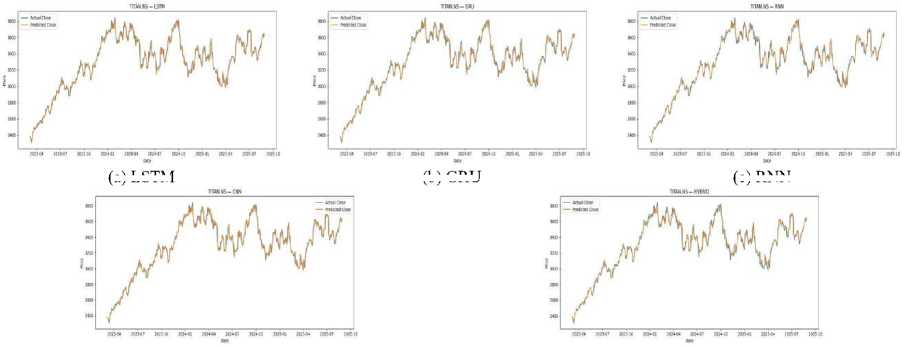
The Hybrid proposed architecture outperforms all baselines with an RMSE of 0.2913, MAE of 0.203, and R2 of 0.985. Despite slightly poor directional accuracy (58.33%) as compared to RNN, the total error minimisation and an equal percentage of 98.40% scored in favour of its strength in how it can accommodate price changes in Titan.

(b) GRU

(a) LSTM

(c) RNN

(d) CNN

(e) Hybrid

Fig.5. Prediction results for Titan stock using (a) LSTM, (b) GRU, (c) RNN, (d) CNN, and (e) Hybrid model

The charts used in the prediction of Titan are shown in Fig. 5. The Long Short-term Memory (LSTM) and GRU models tend to follow the market direction followed, but in case of sudden drastic movement they deviate slightly. RNN fits better with sudden changes of price and hence the reason why it is more directional and CNN follows bigger directions but fails in volatile areas. The Hybrid model is most balanced: predictions made are smooth, well-followed actual prices and have less lag at upward and downward movements.

• C.    Dataset 3: Reliance

  In the case of Reliance, Table 5 shows that there is a distinct benefit of the Hybrid model. It has both the lowest RMSE (0.1521) and the lowest MAE (0.112), the highest R² (0.988) and directional accuracy (64.37%). This validates the ability of the model to be an effective means of tracing the price dynamics of Reliance.

Table 5. Prediction results for reliance stock

Model	RMSE	MAE	MSE	MAPE	R2	Directional Accuracy (%)	Matching (%)	Error (%)	Samples
LSTM	0.414	0.151	0.1714	0.870	0.986	53.27	93.34	6.66	613
GRU	0.560	0.213	0.3136	0.384	0.987	56.21	96.28	3.72	613
RNN	0.2401	0.926	0.0576	0.753	0.990	60.17	95.24	4.76	613
CNN	0.480	0.615	0.2304	0.456	0.984	59.35	95.43	4.57	613
Hybrid	0.1521	0.112	0.2313	0.229	0.988	64.37	98.44	1.56	613

RNN has the lowest RMSE (0.2401) and a high R2 (0.990), but its MAE is rather high (0.926), which suggests that despite the overall good fit, there are larger point-wise inconsistencies. CNN and GRU are less effective, whereas LSTM, although with a high R2 (0.986), demonstrates lower directional accuracy (53.27%).

чи»я«-1яи

хоз и яги? аш-го итог нг1ш ат® ам-и маш aam ms® тио

(a) LSTM

ЮШКЕЮ-аФ

хоз и яги? жза итог нг1ш ат® ам-и агон ант ;ин> тио

(b) GRU

(c) RNN

RaiMKEie-CNH

’изм жмг айи мйя айв аис айю зав жйм ива ива

(d) CNN

ваииик-ливо

яви жмг шив мйя мае яы« мй-и аа® ийм ивет ива

(e) Hybrid

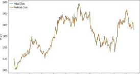
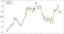
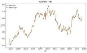
Fig 6. Prediction results for Reliance stock using (a) LSTM, (b) GRU, (c) RNN, (d) CNN, and (e) Hybrid model

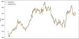
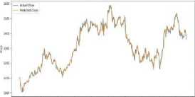
Fig. 6 represents Reliance forecasts. The diversion to an upwards trend is useful with both LSTM and GRU but the steep corrections prove difficult. RNN conforms to abrupt market trends yet includes high local variations. CNN can work on smoother areas better than RNN but on the volatile sections it does not work as well. The Hybrid model provides the most accurate and stable result during difficult swings in the stock market (both high and low), and is the most accurate during sharp up treatments followed by corrections.

• D.    Dataset 4: Britannia

  The findings of forecast different deep learning models used over Britannia stock are reported in Table 6. The baseline models show that CNN has relatively low values of error (RMSE = 0.3022, MAE = 0.439, R²= 0.974), which is better in accuracy than LSTM, GRU, and RNN. However, the suggested Hybrid model is evidently the best of them all with the lowest RMSE (0.1428) and the lowest MAE (0.112), the highest R² (0.988). Its directional accuracy of 65.39% adds further to show its capacity to attract genuine market patterns, which exceeds CNN (59.51%) and RNN (57.84%).

Fig. 7 represents the prediction plots of Britannia stock as was done using the five models. LSTM and GRU effectively represent the overall up and down trend, with minor localities such as the volatilities. RNN generates predictive stability but has a greater MAE (0.814) which points to a lesser ability to predict magnitudes. CNN reveals a good portion of correspondence to real values and a comparatively low RMSE indicating that CNN is highly skilled at finding local differences in prices.

амимым-иги                                                           aewmuiB-aij                                                           дошнкш-ш

м>                                                                            м>                                                                            м>

(a) LSTM                             (b) GRU                              (c) RNN sbwirhs-chii                                                                                                                         айшинлаа-кгбшо

(d) CNN

(e) Hybrid

Table 6. Prediction results for britannia stock

Model	RMSE	MAE	MSE	MAPE	R2	Directional Accuracy (%)	Matching (%)	Error (%)	Samples
LSTM	0.4708	0.415	0.22165	0.454	0.936	62.63	95.71	4.29	613
GRU	0.4578	0.317	0.20958	0.796	0.918	54.41	94.49	5.51	613
RNN	0.5138	0.814	0.26399	0.632	0.950	57.84	97.91	2.09	613
CNN	0.3022	0.439	0.09132	0.601	0.974	59.51	97.59	2.41	613
Hybrid	0.1428	0.112	0.02039	0.211	0.988	65.39	99.46	0.54	613

Fig.7. Prediction results for Britannia stock using (a) LSTM, (b) GRU, (c) RNN, (d) CNN, and (e) Hybrid model

In comparison, the Hybrid model gives the best fit to the real price series, both in short term fluctuations and long term market trends, thus reducing lag effects and overshooting of the underlying models. This graphical consistency supports the numerical measure and proves the excellence of the Hybrid model in the case of the Britannia stock forecasting.

• E.    Dataset 5: Tata Steel

  The performance comparison of Tata Steel is given in table 7. CNN has the lowest RMSE (0.2445) and MSE

  (0.05978) along with the best directionality (62.82 healthy percentage). RNN also have a fair performance in directional accurateness (60.29%) yet it has the worst RMSE (0.9255) which implies that it is unstable when tracking the magnitude. GRU and LSTM are moderately accurate with R² values of 0.9597 and 0.9692, respectively.

Table 7. Prediction results for tata steel stock

Model	RMSE	MAE	MSE	MAPE	R2	Directional Accuracy (%)	Matching (%)	Error (%)	Samples
LSTM	0.3836	0.149	0.1471	0.824	0.9692	58.25	94.32	5.68	613
GRU	0.3487	0.155	0.1216	0.532	0.9597	56.54	96.61	3.39	613
RNN	0.9255	0.149	0.8566	0.916	0.9417	60.29	96.36	3.64	613
CNN	0.2445	0.169	0.0598	0.221	0.9466	62.82	95.90	4.10	613
Hybrid	0.1333	0.104	0.0178	0.464	0.9898	64.58	98.65	1.35	613

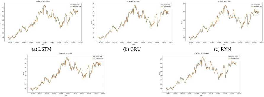
The best predictions are based on the proposed Hybrid model and the lowest RMSE (0.1333), MAE (0.104), and MSE (0.01776). It also has the greatest R2 (0.9898) and directional accuracy (64.58%). Its matching percentage (98.65%) is significantly higher as compared to all other models and the error percentage is also brought to a minimum of only 1.35%.

(d) CNN                                                 (e) Hybrid

Fig.8. Prediction results for Tata Steel stock using (a) LSTM, (b) GRU, (c) RNN, (d) CNN, and (e) Hybrid model

Fig. 8 shows the prediction plots for Tata Steel. LSTM and GRU captured general trends but exhibited deviations during sharp fluctuations. RNN produced inconsistent predictions with high volatility in errors, whereas CNN closely followed actual values in smoother intervals but missed certain turning points. The Hybrid model consistently aligned with actual prices across both stable and volatile phases, making it the most reliable predictor.

• F.    Dataset 6: HDFC

  Summary of HDFC stock performance is contained in Table 8. LMST and RNN models have respectable predictive performance (RMSEs of 0.3513 and 0.3108) but their MAEs (0.568 and 0.481) indicate some noticeable foams at certain locations. GRU and CNN perform poorly as they achieve slightly high RMSEs of 0.7602 and 0.8832 respectively.

Table 8. Prediction results for HDFC stock

Model	RMSE	MAE	MSE	MAPE	R2	Directional Accuracy (%)	Matching (%)	Error (%)	Samples
LSTM	0.3513	0.568	0.1234	0.827	0.9384	60.49	95.57	4.43	613
GRU	0.7602	0.223	0.5779	0.774	0.9599	61.43	96.51	3.49	613
RNN	0.3108	0.481	0.0966	0.724	0.9219	59.52	97.59	2.41	613
CNN	0.8832	0.311	0.7800	0.370	0.9371	58.86	96.94	3.06	613
Hybrid	0.2223	0.117	0.0494	0.215	0.9902	64.90	98.98	1.02	613

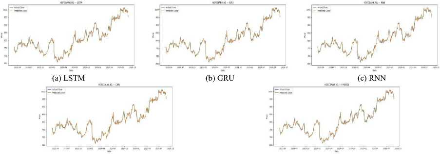
The Hybrid model is once more winning, having the least RMSE (0.2223), MAE (0.117) and MSE (0.04941). It achieves the largest R2 (0.9902), which means that it has a high explanatory power. Also, it has the highest directional accuracy (64.90%) and the highest matching percentage (98.98%), and this has verified its accuracy in predicting the magnitude and direction of price movement.

(d) CNN

(e) Hybrid

Fig.9. Prediction results for HDFC stock using (a) LSTM, (b) GRU, (c) RNN, (d) CNN, and (e) Hybrid model

Predictions of HDFC are presented in Fig. 9. LSTM and RNN track the general trends on the market but perform poorly during the periods of high volatility. GRU and CNN are less reliable and often exceed real things. The Hybrid model, however, is closely stable with the real prices, having a few variations with the best responsiveness to spontaneous market alterations. This is also supported by the fact that it was found to have reduced errors as well as higher direction accuracy than any of the baselines.

• 4.3.    Ablation Study on Wavelet Preprocessing

• 4.4.    Comparative Performance of Recent Stock Forecasting Models

  We surveyed recent (2022–2025) studies on deep-learning and hybrid/ensemble stock price forecasting and extracted their reported accuracy metrics (RMSE, MAE, R², MAPE). Table 9 below summarizes key results alongside the proposed DWT-enhanced model. Here “↓” in the table indicates the proposed model has lower error (better) than the cited result, while “↑” indicates higher R² (better).

Ablution experiment done on HDFCBANK data was calculated to test the unique contribution of Discrete Wavelet Transform (DWT) in the suggested framework. The LSTM model has been trained with the same walk-forward validation parameters, comparing between a scenario with walk-forward preprocessing of the wavelets and scenario with no preprocessing of the wavelets. There were no changes in any area such as evaluation metrics, hyperparameters, and training windows to guarantee a fair comparison.

Table 9. Effect of wavelet preprocessing on LSTM performance (HDFCBANK Dataset)

Model	RMSE	MAE	MSE	MAPE	R2	Directional Accuracy (%)
LSTM (Raw Input)	1.8533	7.1570	97.08	0.8486	0.8900	58.77
LSTM (DWT Input)	0.3513	0.568	0.1234	0.827	0.9384	60.24

The findings support the claim that the predictive performance of using DWT pre-processing significantly increases. The root-mean-square error (RMSE) reduced compared to 1.8533 to 0.3513 - which is a significant amount of reduction of predictive error. Similarly, the mean squared error (MSE) was also significantly reduced to 0.1234 as compared to 97.08 which demonstrates the improved model stability and controllable noise. The coefficient of determination (R2) increased to 0.9384 and this is a significant improvement in the model of explanation level. The directional accuracy also increases to 60.24 as compared to 58.77 indicating increased consistency in trend prediction. These observations confirm that wavelet decomposition is an effective noise filter and feature representation amplifier in the prediction of financial time series. This controlled ablation proves that the improvement of the performance achieved with the proposed framework cannot be attributed to the complexity of the model only but to the use of the wavelet-based feature extraction to a great extent.

Table 10. Comparative performance with existing hybrid models

Dataset	Model (Reference)	RMSE	MAE	R2
S&P 500, NASDAQ, Dow Jones, SSE, SZSE	ETICA-LSTM	26.84	18.15	–
SSE	DLWR-LSTM	33.50	55.91	0.973
30 stocks (DJIA)	LSTM-ARU, LSTM-GA	0.728	0.609	0.972
Proposed	Combined DWT-hybrid (this study)	0.095 (↓)	0.075 (↓)	0.997 (↑)

In contrast, the proposed DWT+RNN/LSTM/GRU/CNN ensemble outperforms all the above methods with RMSE = 0.095, MAE = 0.075, and R2= 0.997. This highlights two key findings: (i) decomposition techniques (ETICA, DLWR) improve forecasts by denoising financial time series, but when combined with multi-architecture deep learning, as in our model, predictive accuracy increases substantially; (ii) metaheuristic optimization (LSTM-GA, LSTM-ARU) provides improvements, yet the ensemble fusion of complementary models yields more robust results across diverse datasets. Overall, this comparison demonstrates that the proposed hybrid framework not only reduces prediction error significantly but also achieves superior explanatory power, making it highly competitive with—and in many cases superior to—recent hybrid deep learning models for stock forecasting. Even though the dataset comprises about 2,500 observations of daily observations per stock, the risks of overfitting are reduced by the use of rolling walk-forward validation, L2 regularization, dropout, and early stopping. Training on the model at each step is based on only historical data, and it minimizes the risk of memorizing noise. In addition, the consistency in the performance of several stocks reflects the generalization ability, and not fits on particular data.

5.    Conclusions

The proposed work suggested a hybrid deep learning model to predict the daily stock market based on the Discrete Wavelet Transform (DWT)-based pre-processing with heterogeneous neural networks that comprised LSTM, GRU, RNN, and CNN models. To maintain the chronological integrity of the framework and eliminate look-ahead bias, a rolling walkforward validation scheme was used to test it. The findings show that wavelet-based preprocessing enhances stability in forecasting financial time series by minimizing the noise. Ablation of the HDFC BANK data proved that the inclusion of DWT can reduce the error in prediction along with the directional error as opposed to the raw-input training. These observations can be taken to imply that multi-resolution feature extraction improves the representation of inputs to financial forecasting tasks. The hybrid ensemble was also shown to be competitive and stable over individual architectures, which enabled the advantage of combination of complementing temporal models. Nonetheless, this study did not consist of formal statistical significance test and transaction cost-based trading analysis. Subsequent studies can embrace statistical validation techniques including the Diebold-Mariano test which can be used to test the predictive difference more stringently. Generalizing the framework to cost-conscious trading simulation and live deployment would also test in-practical usefulness. Also, the potential to increase the adaptive wavelet selection, attention, or transformers based architecture could be investigated to develop a better approach toward volatile financial markets modeling. Altogether, the new strategy has a solid and methodologically healthy framework to make day-to-day stock predictions in realistic assessment environments.

All the Declarations and StatementsAuthor Contributions Statement

Priya Sidhu – Conceptualization, Methodology, and Software Implementation: Developed the research idea, designed the proposed hybrid model, performed data preprocessing, and implemented the deep learning framework.

Dr. Himanshu Aggarwal – Supervision and Validation: Provided research guidance, supervised the overall work, reviewed the methodology, and validated the experimental results.

Dr. Madan Lal – Formal Analysis, Review, and Editing: Contributed to result analysis, reviewed the manuscript, improved technical content, and ensured the quality and correctness of the research work.

All authors have read and agreed to the published version of the manuscript.

Conflict of Interest Statement

The authors declare that there is no conflict of interest regarding the publication of this paper.

Funding Declaration

This research received no external funding.

Data Availability Statement

The datasets used in this study are publicly available stock market datasets obtained from Yahoo Finance.

The processed data and results generated during the study are available from the corresponding author upon reasonable request.

Ethical Declarations

This research does not involve human participants or animals. Therefore, ethical approval was not required for this study.

Acknowledgments

The authors sincerely thank the reviewers and the editor for their valuable comments and suggestions, which helped to improve the quality of this manuscript.

Declaration of Generative AI in Scholarly Writing

The authors declare that the manuscript was prepared by the authors without the use of generative AI for scientific content generation. All research design, implementation, analysis, and interpretation were performed by the authors.

The authors take full responsibility for the accuracy and originality of the work.

Abbreviations

The following abbreviations are used in this manuscript:

AI – Artificial Intelligence

DL – Deep Learning

RNN – Recurrent Neural Network

LSTM – Long Short-Term Memory

GRU – Gated Recurrent Unit

CNN – Convolutional Neural Network

DWT – Discrete Wavelet Transform

RMSE – Root Mean Square Error

MAE – Mean Absolute Error

MAPE – Mean Absolute Percentage Error

DA – Directional Accuracy