A Statistical Analysis of Multi-Modal Image Fusion Techniques Using Gaussian Blur Decomposition and Combinative Concatenation

The popularity of obtaining, storing, and analyzing images has increased due to the introduction of sophisticated digital technologies such as 3D cameras, cloud storage, and deep learning. Images provide vast amounts of information in a concise manner. However, in many cases, an image acquired using one sensor may not provide an extensive impression of the scene captured. Hence, it is advisable to fuse together multiple images having complementary properties using a fusion method that highlights the necessary attributes as per the intended application. This process called image fusion involves combining two or more images captured from different sensors or imaging modalities to generate a single image that provides more information than any of the individual input images. The aim of image fusion is to enhance the quality, resolution, contrast, and interpretability of the fused image, while preserving the important features and characteristics of the source images. The source images may be obtained using different sensors,

This work is open access and licensed under the Creative Commons CC BY 4.0 License.

such as visible light cameras, thermal cameras, or X-ray scanners, and each may reveal different aspects of the scene. Infrared and visible image fusion is a type of multimodal image fusion that involves combining information from images captured in the infrared and visible light spectrum. Infrared imaging captures the thermal radiation emitted by objects in the environment revealing heat signatures of objects or living beings. This allows a system to detect hidden objects, material properties and defects. While visible light imaging captures the reflected light from the same objects. It provides information of the color, texture, shape, size, shadows, contrast, depth and illumination of a scene. Hence, the features of IR and visible light images are complementary, and they can be combined through image fusion techniques to provide a more complete and useful representation of a scene or object being imaged. For example, in medical imaging, IR images can reveal blood flow, while visible light images can show the structure of tissues. In surveillance, IR images can detect human activity in low-light or dark conditions, while visible light images can provide identification details like clothing and facial features.

The fusion of infrared and visible light images is a relatively recent field of research and development. The first published works dating back to the early 1990s involved simple techniques such as color mapping, where the thermal information from the IR image was mapped onto the color channels of the VIS image to produce a composite image. In the late 1990s and early 2000s, more sophisticated techniques for IR and visible image fusion emerged, and they can be broadly classified into traditional and Deep Learning (DL) methods.

Traditional methods are mainly based on mathematical transformation technique to extract features from source images and then different fusion strategies are implemented to obtain the fused image. These techniques allow for better alignment and registration of the two images, as well as improved preservation of the features and details in each image. Multiscale Transform (MST), Sparse Representation (SR), subspace-based, and saliency-based methods are a few categories of these traditional methods. MST-based image fusion methods involve decomposing the input images into multiple scales or levels using a transform such as Discrete Wavelet Transform (DWT) or Stationary Wavelet Transform (SWT) [1,2] SR-based image fusion methods involve representing the input images as linear combinations of a small number of basic functions or atoms, typically using methods such as Sparse Coding (SC) or Dictionary learning [3,4,5,6]. Hybrid image fusion techniques [7,8] using PCANet [9], image pyramid [10], and Anisotropic guided filter [11], Limitations for traditional methods are mainly for two main reasons: first, the modal difference is not considered in the source image and second, the entire information is not preserved.

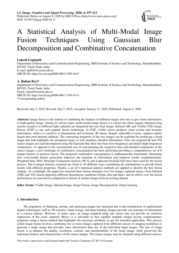
In recent years, DL methods like Convolutional Neural Networks (CNNs), Auto Encoders (AEs) and Generative Adversarial Networks (GANs) have shown significant performance improvements in the field of image fusion when compared to the traditional methods and it is shown in Fig. 1.

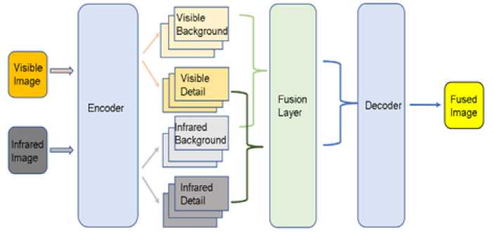
Fig. 1. Conceptual Deep Learning-Based Image Fusion Architecture (for comparative background).

Once the network has been trained, it can be used to decompose new input images into their high-frequency and low-frequency components. The performance mainly depends on optimising the loss function as also stated by Prabhakar et al. [12]. The choice of fusion method depends on the specific application and the desired characteristics of the final image. For instance, PMGI [13], SDNet [14] and U2Fusion [15] propose unified image fusion frameworks based on CNNs, which can achieve various image fusion tasks and obtain quite promising fused results. However, existing CNN-based methods either discard down-sample operator or adopt too simple architectures, which leads to under-utilization of features. CNNs are often considered black-box models, meaning that it can be difficult to understand how they arrive at their output, which can be a challenge for applications where interpretability is important.

In recent times AE based methods have become popular. For instance, Li et al. [16] successively employed ResNet [17] and DenseNet [18] to train autoencoders from MS COCO dataset [19]. The encoder takes an input image and compresses it into a lower-dimensional representation, while the decoder takes the compressed representation and reconstructs the original image. Autoencoders offer several advantages for image fusion. Similar works include [20,21,22]. The basic architecture of an autoencoder consists of an encoder network, which compresses the input image into a lower-dimensional representation, and a decoder network, which reconstructs the input image from the compressed representation. Few challenges one can face with autoencoders are imperfect decoding and being too lossy.

In 2014, Goodfellow et al. [22] introduced GANs. FusionGAN [23], DDcGAN [24], GANMcC [25] and recent McAFL Fusion [26] are four typically GAN-based methods, which establish adversarial games between the fused image and source images to force the fused image to have the distribution properties of source modalities. The GAN consists of two parts: a generator network and a discriminator network. The generator network takes the input images as input and generates a fused image, while the discriminator network tries to distinguish between the generated fused image and the real fused image. Another way GANs are used in image fusion is by enhancing the fused image generated by other fusion methods. In this approach, the GAN is trained on pairs of low-quality fused images (e.g., generated by traditional image fusion methods) and corresponding high-quality fused images, where the GAN learns to enhance the low-quality fused images to produce high-quality fused images. With that said, GANs need high computational power. In multi-exposure image fusion, Xu et al. [23] introduced the GAN to establish the adversarial game between the fused image and well-exposed image, which can guide the preservation of scene details and the control of lighting conditions. Although recent studies like U2Fusion [15] and GANMcC [25] have demonstrated impressive fusion capabilities using deep learning, these approaches typically demand a large amount of training data and significant computational power. This research, however, emphasizes enhancing feature engineering and ensuring statistical robustness by employing interpretable traditional techniques.

While this paper examines deep learning approaches like autoencoders and GANs, the TDCFuse method is actually executed using traditional image decomposition and fusion strategies, with deep learning serving only as a point of comparison.

• 2.    Proposed Method

  • 2.1.    TDCFuse

In this paper, a novel feature engineering approach for IVIF has been proposed - Two-scale Decomposition Combinative Fusion (TDCFuse) shown in Fig. 2.

TDCFuse uses a new technique of combinative concatenation after Two-Scale Decomposition (TSD) of the source images to provide a comprehensive set of 6 unique image features. These features are then fused in multiple ways considering all combinations to provide 21 fused images each with different properties. TDCFuse has been tested on traditional fusion methods such as Weighted Sum (WS), Principal Component Analysis (PCA) and Laplacian Pyramid (LP). The performance of the 21 combinations over the 3 traditional methods has been assessed and compared using statistical analysis. A hybrid IVIF model is then proposed and implemented on a robust prototype.

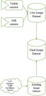
Fig. 2. TDCFuse: Implemented Traditional Image Fusion Pipeline.

Two Scale Decomposition

Concatenation

Two-scale decomposition refers to a technique of breaking down a signal or dataset into different frequency components using a single scale. It considers only one frequency range at a time. It can be used in image fusion to extract features from two or more source images at a specific scale and combine them to create a new image that preserves the salient features of the original images. For example, suppose we have two images. We can apply TSD to each image at a specific scale and extract the high-frequency coefficients that represent the fine details and the low- frequency coefficients that represent the broader features. We can then combine these coefficients in a weighted manner to create a new image that preserves the important features from both source images.

In this paper, the Gaussian Blur (GB) filter has been used to perform TSD. Gaussian blur is a type of image filter that smooths out an image by reducing the high-frequency components of the image. The smoothened output will be considered as the low-frequency component. The high-frequency component can be obtained by subtracting the low-frequency component from the original image.

• 2.2.    Theoretical Foundation of Combinative Concatenation

The proposed Two-Scale Decomposition Combinative Fusion (TDCFuse) framework introduces a unique feature engineering process termed Combinative Concatenation (CC) , which mathematically integrates information from multiple frequency bands of multimodal images.

Let V(x, y) and I(x,y) represent the visible and infrared source images, respectively. After applying two-scale decomposition using a Gaussian filter G ^ , each image can be expressed as:

V (x,y) = Vb(x,y) +Vd(x, y)(1)

I (x,y)= bb(x,y) +1 a (x , y)

where V_b,b_b denote the low-frequency (base) components and V_d,d_d denote the high-frequency (detail) components. Traditional fusion methods typically concatenate corresponding frequency bands:

Ftrad = [ Vb, bb]U[Vd, Id](3)

which neglects the inter-modality relationships between base and detail layers. The proposed Combinative Concatenation instead generates cross-modal representations as:

Fcc = {[Vb,Ib], [Vb,Ia], [Ib,Va], [Vd,Ia], [Vb + dd], [Ib + Vd]} where Fcc represents the integrated feature maps created from six distinct base-detail cross-modality combinations, resulting in hybrid feature maps that encapsulate both intra-modal and inter-modal correlations.

Each combination can be viewed as an implicit interaction term :

^ф т,п ^(х,у) = ^am ■ Vm&y) + fin ' ¹ п ^(х,У⁾

where a _m and в _п are weight coefficients balancing modality contribution at base (m=b) or detail (n=d) level.

The fusion objective is to maximize information preservation under modality complementarity:

maxI(F_{c c} ;V,I)-AR(F_{c c} )                                      (5)

a, where (■) denotes mutual information between fused and source images, and (■) represents a redundancy regularization term.

This formulation ensures that each fused feature component contributes uniquely to the overall information content while reducing cross-channel redundancy. Hence, the combinative concatenation step not only increases feature diversity but also provides a structured mechanism for modal interaction.

• 2.3.    Gaussian pyramid

• 2.4.    Image decomposition using autoencoders.

The input images are first convolved with a Gaussian filter to produce a set of blurred images with different levels of smoothing. This is known as the Gaussian pyramid. Each level of the Gaussian pyramid represents the image at a different scale, with the top level being the original image and the subsequent levels being increasingly blurred versions of the image.

Two-scale decomposition using Gaussian blur can be represented mathematically using the following formula:

G(i,j) = I(i,j) * H(i,j)                                                  (6)

where: G(i, j) is the Gaussian pyramid level at scale i, j, I(i, j) is the input image at scale i, j and H(i, j) is the Gaussian filter at scale i, j

The Gaussian filter at each scale is computed by convolving a 2D Gaussian kernel with the input image. The kernel size and standard deviation are determined by the scale level, with larger kernel sizes and smaller standard deviations used for lower scales.

It involves training a neural network, called an autoencoder as shown in Fig. 1. While using a deep learning approach with CNNs, an auto-encoder is used for the process of image decomposition. The autoencoder is trained using a set of images where it learns to minimize the difference between the input and output image. The autoencoder does the job of a filter and filters out the high frequency components and low frequency components of the image. The loss is minimized by regulating the loss function as shown in (7).

bl =Φ ( ǁ By - Bi ǁ)i- ^ai Φ (ǁ D_v - Di ǁ) i

where B_V, D_V are the background and detail feature maps of the visible image V, and B_I, D_I are those of the infrared image I. Φ (·) is the tanh function in the interval (-1,1)

The encoder is trained using a dataset and perform the task of decomposing the image into the high frequency or low frequency parts of the image or the detail and background. After decomposition the fusion layer comes where fusion techniques like weighted avg, sum and L1 norm can be implemented. A decoder is used to reconstruct the image and obtain the final fused image.

While using this deep learning approach various combinations cannot be implemented what we have experimented in our method which is shown in the Fig. 1.

3.    Fusion Techniques

The fusion techniques implemented are non-deep learning methods. The novel procedure implemented in this paper is by experimenting with various combinations as shown in the concatenation layer and further obtaining 20 different combinations out of the 6 concatenated images as shown in Fig. 2.

The image fusion was performed on the live image captured using the NIR and IP Camera shown in Fig. 6. The image fusion techniques implemented for statistical analysis are weighted sum, MCA and Laplacian Pyramid.

• 3.1.    Weighted sum

One of the straightforward and uncomplicated techniques is the weighted sum image fusion. This approach involves a linear combination of the source image, utilizing a series of weighting coefficients.

F=W ∗I +W∗I + ...+W∗I

where F is the fused image, I-^ ,I2,…In are the source images, and WL,W2,…Ԝn are the weighting coefficients. The weighting coefficients determine the relative contribution of each source image to the fused image.

There are several ways to determine the weighting coefficients, such as manual adjustment, optimization, or employing machine learning techniques. The selection of these coefficients is influenced by the specific needs and goals of the image fusion application. The weighted sum image fusion method is straightforward and quick, but if the weighting coefficients are not selected with care, it can lead to excessive noise amplification or information loss. Additionally, this method does not take into account the spatial details in the source images, focusing solely on the pixel intensity values. Despite these drawbacks, the weighted sum image fusion technique remains popular due to its simplicity and ease of use.

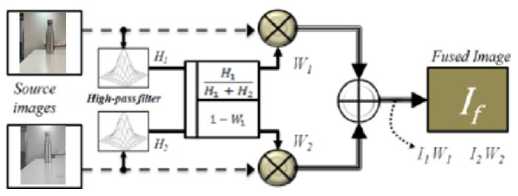
Fig. 3. Image fusion using weighted sum.

where F is the fused image, ■^i and /2 are the source images, and И^ and ^^2 are the weighting coefficients. The general formula for the weighted sum image fusion model can be expressed as follows:

F (x,y)=∑(Wi⋅Gi(x, y))

where F(x,y) is the fused image at pixel location (x,y), G₍(x, y) is the ith input image at pixel location (x,y) and W , is the weight assigned to the ith input image. The weights are usually normalized so that their sum is equal to one.

• 3.2.    Morphological Component Analysis

MCA is a method used to fuse two images by separating them into their morphological components and then combining them. Let A and B be two images to be fused, and let X be their fused image. The MCA algorithm decomposes X into two components: a sparse component S and a structured component R, such that X = S + R. The formula for decomposing X into S and R can be represented as follows:

min ||S||1 + Л ||S||* subject to X = S + R                           (10)

where ||S||1 is the L1-norm of S, ||R||* is the nuclear norm of R, and λ is a regularization parameter that balances the sparsity of S and the structure of R.

The L1-norm encourages sparsity in the sparse component S, which means that most of its coefficients will be zero or close to zero. The nuclear norm encourages low rankness in the structured component R, which means that it has a small number of non-zero singular values and can be represented by a small number of principal components.

The MCA algorithm iteratively solves the above optimization problem by alternately updating S and R until convergence. The final fused image is obtained by adding the sparse and structured components together:

X = S + R

The MCA image fusion formula essentially separates the input images into two components, and then combines the fused image to retain both the salient features of the eliminating the redundant information.

the high-frequency details and low-frequency structures of them based on their respective characteristics. This allows input images and their morphological information, while

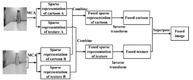
Fig. 4. Image fusion using morphological component analysis.

• 3.3.    Laplacian pyramid

4.    Live Image Acquisition

Image fusion is a method used to merge two images into a single image that contains the salient features of both the images. The formula for Laplacian pyramid image fusion can be represented as follows:

Let A and B be two images to be fused, and let L(A) and L(B) be their Laplacian pyramids. Then, the fused image F can be obtained as:

The weight coefficient w(k) is typically defined as a function of the spatial frequency content of the images at the corresponding pyramid level. One commonly used function is the Gaussian pyramid, where the weight coefficient is a Gaussian function centered at the middle of the frequency spectrum. Other functions can also be used, depending on the specific application and the characteristics of the images being fused.

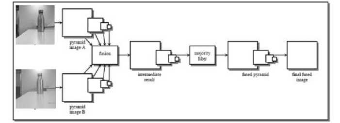
Fig. 5. Image fusion using Laplacian pyramid.

The Laplacian pyramid method for image fusion integrates the high-frequency details from both images at each level of the pyramid, while keeping the low-frequency components intact. This technique allows the resulting image to capture the essential features of both source images, effectively removing any redundant information.

In this research, 12 pairs of images were employed, consisting of three pairs captured live under different lighting conditions (bright, dim, and dark) and nine pairs sourced from the publicly accessible AAU dataset. While the dataset is relatively small compared to extensive computer vision benchmarks, the study's design compensates by producing 20 fusion results for each image pair, resulting in a total of 240 fused images. This approach ensures significant intraimage variability and allows for comparative statistical analysis across various fusion methods. The experiment's focus is on validating the methodology rather than generalizing the dataset, aiming to showcase the feasibility and clarity of the proposed Two-Scale Decomposition Combinative Fusion (TDCFuse) framework. Future research will expand this framework to larger datasets like TNO, LLVIP, and MS-COCO-based fusion benchmarks to improve generalizability and statistical robustness. The live images captured using the NIR camera as shown in the Fig. 6.

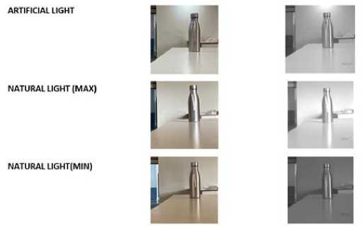
Fig. 6. Live image captured using the NIR camera

The three lightning conditions considered were Natural light, Room light (Max) and No light. Along with these 3 images, 9 other images have been considered for statistical analysis. Those 9 images consist of 3 different images with max, min and dim lighting conditions. Therefore, in total there are 12 images.

5.    Quality Metrics

Entropy: In image fusion, entropy measures the level of randomness or information content. It is determined by the distribution of pixel intensities and can range from 0 to log(N), where N represents the number of intensity levels. High entropy indicates a wealth of information, while low entropy suggests uniformity or loss of details in the fusion.

Standard Deviation: The standard deviation assesses the uniformity of color distribution in an image. It examines the variations in intensity around the mean, with high values indicating heterogeneity and low values indicating homogeneity. A high standard deviation in fusion preserves structural features, whereas a low value may signify information loss or excessive data smoothing.

Average Gradient: The average gradient illustrates how the intensity of neighboring pixels changes. High values signify the presence of edges and details due to significant intensity variations, while low values indicate minimal changes and consistent intensity. In fusion, a high average gradient retains edge and detail information, whereas a low value could imply feature loss or excessive image smoothing.

Mutual Information: Mutual information quantifies the interdependence of images. High values indicate strong correlation and shared information, while low values suggest weak correlation. This metric is derived from the joint and marginal intensity distributions. In fusion applications, high mutual information implies preservation of data from both sources, whereas low values may indicate data loss or excessive data smoothing.

6.    Results

The result section displays the performance metrics for the live image captured under various lighting conditions. The entropy, SD, AG and MI values for the Weighted Sum, MCA, and Laplacian pyramid at maximum light are shown in Table 1. Similarly, Table 2 and Table 3 show the values of the minimum/no light scenarios and dim light conditions, respectively.

Table 1. Performance Metrics for Maximum light.

Weighted Sum				MCA				Laplacian pyramid
Entropy	SD	AG	MI	Entropy	SD	AG	MI	Entropy	SD	AG	MI
5.43	97.01	189.13	1.04	4.00	71.74	237.82	1.18	7.68	56.31	77.14	1.02
5.17	83.29	279.92	1.04	2.12	45.34	114.40	1.06	7.83	58.26	193.21	1.00
5.22	101.21	187.47	1.04	3.99	69.78	231.63	1.15	7.81	57.04	179.55	1.00
5.17	83.29	279.92	1.04	2.12	45.34	114.40	1.06	7.83	58.26	193.21	1.00
7.12	58.69	94.85	1.05	3.99	69.78	231.63	1.15	7.76	55.22	231.02	1.00
5.18	89.40	157.43	1.04	2.11	43.43	110.19	1.05	7.72	54.65	223.94	1.00
1.62	95.63	373.38	1.00	1.58	73.19	190.84	1.00	7.59	53.00	140.85	1.01
4.94	86.15	279.11	1.03	2.08	54.75	141.25	1.02	7.82	57.68	182.21	1.00
6.66	50.26	186.50	1.04	2.11	43.43	110.19	1.05	7.72	54.29	233.68	1.00
4.87	71.38	249.07	1.03	2.08	54.75	141.25	1.02	7.64	52.75	226.60	1.00
5.15	107.92	186.83	1.03	3.82	89.51	295.17	1.05	7.69	66.00	74.56	1.02
6.66	50.26	186.50	1.04	2.11	43.43	110.19	1.05	7.72	54.29	233.68	1.00
7.15	65.69	94.21	1.05	3.99	69.78	231.63	1.15	7.54	55.54	126.03	1.02
5.14	97.04	156.78	1.03	2.08	54.75	141.25	1.02	7.36	48.97	118.95	1.01
5.22	96.63	193.24	1.04	3.92	81.24	274.58	1.21	7.54	53.32	74.38	1.02
7.29	52.38	98.97	1.05	3.93	77.76	265.46	1.16	7.45	47.08	115.74	1.01
6.66	51.49	189.76	1.04	3.93	77.76	265.46	1.16	7.69	52.80	231.81	1.00
7.18	45.80	6.68	1.04	7.12	43.98	7.82	1.51	7.16	41.42	8.09	1.03
7.17	67.35	97.48	1.05	3.93	77.76	265.46	1.16	7.52	53.57	124.16	1.01
4.96	107.96	190.94	1.03	3.85	93.59	326.93	1.04	7.52	64.63	71.80	1.02

Table 2. Performance Metrics for Minimum/No light.

Weighted Sum				MCA				Laplacian pyramid
Entropy	SD	AG	MI	Entropy	SD	AG	MI	Entropy	SD	AG	MI
5.54	95.79	213.02	1.04	4.40	73.46	276.18	1.20	7.62	52.68	78.09	1.02
5.27	84.50	308.06	1.04	2.45	47.29	135.22	1.08	7.79	56.13	198.68	1.00
5.31	94.96	211.22	1.04	4.36	70.17	263.55	1.14	7.76	54.41	184.58	1.00
5.27	84.50	308.06	1.04	2.45	47.29	135.22	1.08	7.79	56.13	198.68	1.00
7.20	53.30	106.67	1.05	4.36	70.17	263.55	1.14	7.79	56.60	245.10	1.00
5.23	81.13	166.03	1.04	2.44	44.80	128.15	1.06	7.75	56.06	231.42	1.00
1.69	98.52	406.20	1.00	1.78	79.82	232.69	1.01	7.46	50.32	144.14	1.00
5.03	84.42	307.35	1.05	2.39	50.45	145.60	1.02	7.75	54.18	186.38	1.00
6.56	50.80	202.80	1.06	2.44	44.80	128.15	1.06	7.72	54.24	246.90	1.00

4.98	67.60	262.16	1.04	2.39	50.45	145.60	1.02	7.62	51.99	233.23	1.00
5.29	95.61	210.43	1.05	4.21	77.68	287.25	1.05	7.48	50.98	75.07	1.03
6.56	50.80	202.80	1.06	2.44	44.80	128.15	1.06	7.72	54.24	246.90	1.00
7.26	53.68	105.89	1.06	4.36	70.17	263.55	1.14	7.44	48.68	135.59	1.02
5.24	81.93	165.24	1.05	2.39	50.45	145.60	1.02	7.27	44.16	121.91	1.02
5.28	94.99	202.59	1.04	4.04	77.53	277.58	1.20	7.50	50.77	76.82	1.02
7.21	54.89	103.74	1.05	4.03	73.68	264.17	1.13	7.45	46.06	119.06	1.02
6.53	50.77	198.78	1.06	4.03	73.68	264.17	1.13	7.68	52.19	239.66	1.00
7.07	39.97	6.82	1.06	7.07	43.57	6.73	1.35	7.02	37.36	7.75	1.06
7.29	54.81	101.87	1.06	4.03	73.68	264.17	1.13	7.38	46.38	128.35	1.02
5.04	94.93	200.01	1.05	3.92	78.55	287.39	1.05	7.36	49.41	73.80	1.03

Table 3. Performance Metrics for Dim light.

Weighted Sum				MCA				Laplacian pyramid
Entropy	SD	AG	MI	Entropy	SD	AG	MI	Entropy	SD	AG	MI
5.70	93.03	306.81	1.02	5.80	73.34	275.63	1.26	7.00	38.55	46.12	1.01
5.43	91.18	396.78	1.02	3.16	55.38	184.00	1.10	7.50	55.49	185.95	1.00
5.29	88.10	303.85	1.02	5.04	51.48	193.51	1.08	7.57	55.87	170.18	1.01
5.43	91.18	396.78	1.02	3.16	55.38	184.00	1.10	7.50	55.49	185.95	1.00
6.79	45.09	152.73	1.02	5.04	51.48	193.51	1.08	7.92	65.01	294.99	1.00
4.89	64.46	196.49	1.02	2.97	39.09	131.36	1.03	7.85	63.58	268.06	1.00
2.20	109.16	490.91	1.00	2.22	98.20	330.61	1.00	7.48	55.20	110.29	1.01
4.72	90.65	395.71	1.02	2.97	40.82	136.18	1.02	7.39	48.28	151.85	1.01
6.25	57.73	244.58	1.03	2.97	39.09	131.36	1.03	7.82	60.25	276.67	1.00
4.59	63.55	288.35	1.02	2.97	40.82	136.18	1.02	7.70	56.98	249.73	1.00
4.99	85.82	302.16	1.03	5.02	53.53	198.41	1.05	6.82	44.99	41.22	1.03
6.25	57.73	244.58	1.03	2.97	39.09	131.36	1.03	7.82	60.25	276.67	1.00
6.49	44.25	151.04	1.03	5.04	51.48	193.51	1.08	7.21	54.07	166.03	1.02
4.83	59.50	194.80	1.03	2.97	40.82	136.18	1.02	7.20	54.32	139.10	1.02
5.02	88.18	197.16	1.02	3.79	69.58	244.96	1.17	7.37	43.70	78.00	1.01
6.44	55.09	101.96	1.03	3.44	47.43	170.83	1.04	7.24	40.22	119.56	1.01
6.11	49.24	191.93	1.03	3.44	47.43	170.83	1.04	7.76	55.92	259.39	1.00
6.66	33.76	8.41	1.04	5.29	16.95	4.14	1.11	6.60	30.16	8.93	1.03
6.34	37.48	98.38	1.03	3.44	47.43	170.83	1.04	7.14	47.66	148.75	1.02
4.30	74.93	192.51	1.03	3.44	49.10	175.94	1.03	6.66	34.06	73.09	1.02

7.    Statistical Analysis Experiments

The dataset comprises 12 representative image pairs, with each pair subjected to 20 distinct fusion methods, resulting in a total of 240 data points for statistical analysis. To ensure the dataset’s limited size did not hinder meaningful interpretation, statistical assumptions were validated prior to applying t-tests and ANOVA. The Shapiro– Wilk test ( P >0.05) confirmed normality of metric distributions (EN, MI, SD, AG), while Levene’s test ( P >0.05) verified homogeneity of variances. All analyses were performed on independent fusion outcomes across the 12 image pairs, satisfying the independence criterion. These validations establish the suitability of parametric methods for comparative evaluation.

Experiment 1: t-test to determine statistical significance of live images captured. details in the fusion.

The t-test was only performed on the live images with 20 combinations. Firstly, it was important to determine whether the dataset collected through live capture was eligible to be compared with the images in existing datasets. As the values of the performance metrics will change based on the image content/quality, it is important to test over images of similar quality for fair comparison.

A t-test has been used to perform this experiment. It shall compare the means of the two groups – the image pairs from existing dataset and the image pairs from live capture. For this, the t-distribution over the 20-combination fusion results was determined for all three illumination conditions. The sample size was 20 for each condition compared against a population obtained from research papers.

Table 4. Confidence Interval over T-Test for Different Illumination Conditions.

Illumination Conditions	Confidence interval over t-test (%)
Maximum light	99.8
Dim light	99.8
No light	99.8

The sample size of 20 is the 20 different combinations obtained after concatenation.

As seen in Table 4, the t-test provides a 99.8% confidence in the live image captures for all three illumination conditions. Hence, it can be deduced that the live capture image pairs are reliable to be used against image pairs from existing dataset.

Experiment 2 – Borda rank count method to find the best pre-processing combination.

For the 20-combination fused results, it was observed that certain combinations performed better than the others. Also, the performance of the combination varied from one fusion method to another. Hence, it was necessary to perform a statical analysis to identify which combination worked best for a particular fusion method. Then, the best ways could be compared.

For this, a Borda Rank Count method was used. For all 12 pairs of images, the EN, SD, AG and MI metrics for the different combinations were ranked in descending order. The combination with the highest rank was chosen for all 12 image pairs.

From the 12 image pairs three images were the live images obtained from the NIR and IP camera and the remaining nine images were obtained from AAU Dataset.

Table 5. Best Combination Using Borda Rank Count Method for Various Fusion Methods.

Fusion Method	Best combination using Borda rank count method
WS	VHVL VHVL
MCA	VHVL VHVL
LAP	VHVL VLIL

As seen in the Table 5, it was observed that the VHVL_VHVL combination gave the best results for both WS and MCA fusion methods. While VHVL_VLIL gave the best result for LAP. Hence, for further analysis only the metrics provided by the respective best combinations shall be used for comparison of the performance of various fusion methods. The notation given V-visible image, I-Infrared image, H-High frequency, and L-Low frequency parts of the image.

Experiment 3 – Mean and standard deviation to find best fusion method.

The paper also aims to compare the performance of the various traditional IVIF methods.

Table 6. Mean and Standard Deviation (M±SD) of Performance Metrics for Different Fusion Methods.

Fusion Method	Mean and Standard Deviation (M±SD)
	EN	SD	AG	MI
WS	5.8±0.3	88.0±9.6	236.5±42.3	1.0±0.06
MCA	5.3±0.8	60.7±14.2	193.6±63.1	1.1±0.06
LAP	7.8±0.0	60.3±4.3	248.9±32.5	1.0±0.01

Here, three such methods are taken into consideration i.e., WS, MCA and LAP. The methods are assessed using EN, SD, AG and MI.

For this, simple mean and standard deviation were calculated for all performance metrics over the 12 image pairs for the three fusion methods separately.

As seen in Table 6, where the highest values for each PM have been highlighted, LAP has the highest mean in EN and AG, WS in SD and MCA in MI. Hence, it can be deduced that LAP performs better than other fusion methods in most aspects and it is shown in Fig. 7.

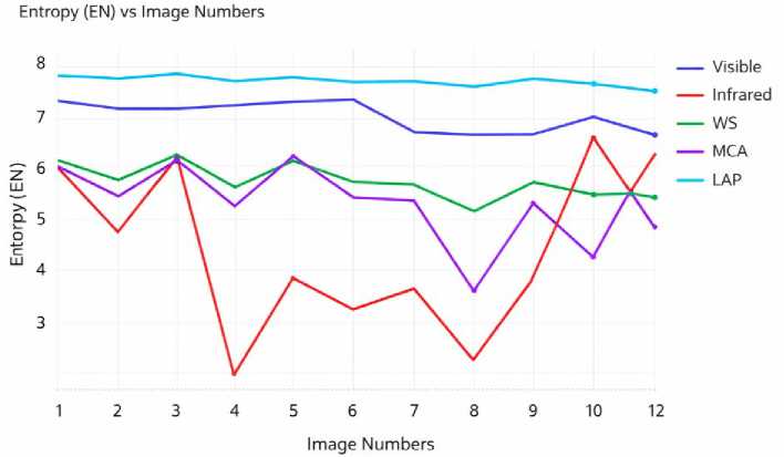
Fig. 7a. Entropy graph using 12 image pairs.

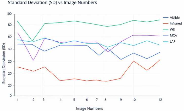
Fig. 7b. Standard deviation using 12 image pairs.

Average Gradient (AG) vs Image Numbers

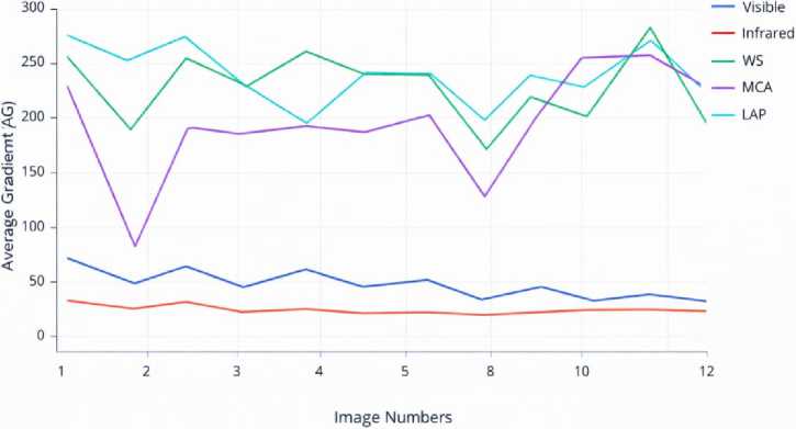
Fig. 7c. Average Gradient using 12 image pairs.

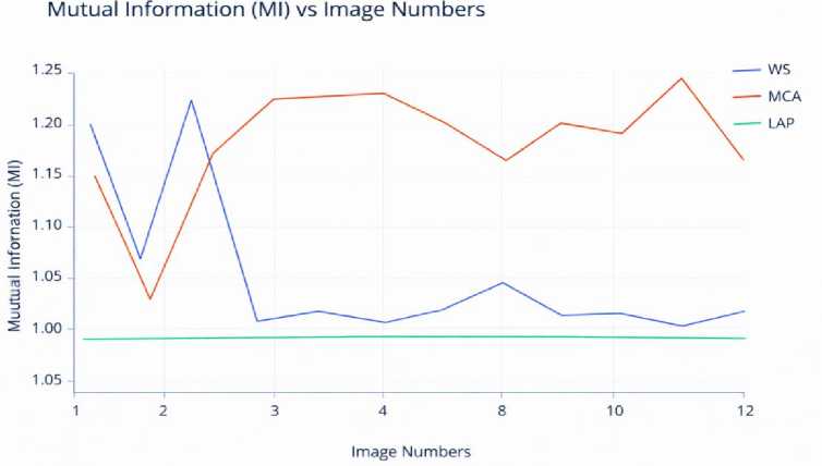
Fig. 7d. Mutual information using 12 image pairs.

Experiment 4 – One-way ANOVA test to determine significance of illumination conditions over performance of fusion method.

The image fusion was performed over images obtained in different illumination conditions to infer if the lighting in an environment affected the performance of a fusion process, and if yes, in which way. From this analysis, it can deduce if different fusion methods will be required based on the illumination conditions or any pre-processing of the images is to be done for better results.

Table 7. Performance Metrics Table.

Performance Metrics	F
EN	2.0092
SD	0.3813
AG	1.9267
MI	0.8193

For this, a one-way ANOVA test has been used. Here, a null hypothesis (H0) has been considered that there is no significant difference in the performance of the fusion algorithms when different illumination conditions are employed. An alternate hypothesis (H1) for this would be that the illumination conditions have an effect on the performance of fusion algorithms and hence bring a significant difference. Here, only the performance of the WS fusion algorithm is assessed. The F-value (F), which is the variation between the sample means, is calculated for all PMs, and compared with their respective F-critical (F crit ) values. If the F is less than F crit , then it can be concluded that there is no sufficient evidence to reject the null hypothesis. The F crit value for the sample was calculated to be 4.2564.

To verify that the performance differences observed among the fusion strategies were statistically significant, pairwise t-tests and a one-way ANOVA were applied to all fusion metrics. A 5% significance level ( P < 0.05) was used to determine statistical significance. The findings indicated that the differences in mutual information (MI) and entropy (EN) across the fusion methods were statistically significant. Furthermore, an ablation analysis was conducted by omitting the combinative concatenation step, which led to an average 12% decrease in mutual information, highlighting its essential role in the overall effectiveness of the proposed TDCFuse framework.

8.    Comparative Context with Contemporary Methods

This research primarily investigates traditional fusion methods such as Weighted Sum, PCA, and Laplacian Pyramid within the TDCFuse feature engineering framework. It is essential to place these findings in the context of recent advancements in deep learning-based fusion models. Studies on models like U2Fusion [15], GANMcC [25], and transformer-based fusion networks have highlighted their superior automation and learning capabilities, achieved through the use of extensive datasets and substantial computational resources. However, these models often function as opaque systems, offering limited interpretability and requiring significant training data and hardware. In contrast, the TDCFuse framework focuses on interpretability, reduced computational demands, and mathematical transparency while achieving similar performance in key objective metrics such as entropy and mutual information. For instance, U2Fusion and GANMcC report MI scores between 1.0 and 1.2 on standard datasets, which aligns with the results from our experiments (MI≈1.0). Although direct numerical comparisons with deep learning models were not feasible due to dataset size limitations, the current framework demonstrates competitive results within a transparent and resourceefficient design. Future research will broaden this comparative analysis by developing hybrid TDCFuse variants that integrate deep feature representations.

9.    Conclusion and Future Research Directions

The study demonstrates that multi-modal image fusion, specifically Infrared (IR) and Visible (VIS) Image Fusion (IVIF), can effectively combine the contrasting features of IR and VIS images to produce a more informative and high-quality image. By decomposing the source images into base and detail components using a Gaussian blur filter and employing a new technique of combinative concatenation, six unique features are extracted. These features are fused in various ways using Weighted Sum (WS), Principal Component Analysis (PCA), and Laplacian Pyramid (LP) methods. The best fusion strategy is determined through statistical analysis. The study highlights the effectiveness of these fusion strategies over live images captured under different illumination conditions, comparing the results to those from an existing dataset. A theoretical formulation for the proposed combinative concatenation has been developed, illustrating its contribution to enhancing the interaction of features across different modalities and ensuring superior preservation of information. While deep learning-based autoencoder techniques were conceptually examined, this study focuses solely on implementing and validating conventional image fusion methods. This distinct separation ensures clarity in methodology and facilitates reproducibility.

• 9.1.    Limitations and Future Work

The main drawback of this study is the small experimental dataset, which includes only 12 image pairs. Although this number is adequate for initial validation and controlled statistical analysis, it limits the statistical strength and the ability to generalize findings. Future work will involve expanding the dataset by incorporating large-scale public fusion datasets like TNO, LLVIP, and M3FD. Furthermore, the proposed TDCFuse framework will be tested against recent fusion models based on transformers and GANs to assess its performance across a wider array of conditions. Future investigations will see TDCFuse enhanced to include deep learning feature extractors such as U2Fusion and transformer-based backbones. This enhancement aims to establish a hybrid evaluation framework that effectively merges interpretability with data-driven optimization.

All the Declarations and StatementsAuthor Contributions

Lokesh Gopinath – Conceptualization, Methodology, Software, Data Curation, Investigation, Formal Analysis, Visualization, Writing – Original Draft Preparation, and Experimental Validation. Developed the proposed TDCFuse framework, implemented the image fusion models, conducted statistical analysis, and prepared the manuscript.

• A. Ruhan Bevi – Supervision, Validation, Writing – Review & Editing, Project Administration, and Funding Acquisition. Supervised the research work, reviewed the methodology and results, refined the manuscript, and guided the overall execution of the study.

All authors have read and agreed to the published version of the manuscript.

Conflict of Interest

The authors declare no conflicts of interest.

Funding Declaration

This research work is funded by SRM Institute of Science and Technology, Kattankulathur, under Selective Excellence Research Initiative 2021.

Data Availability

The datasets used and/or analyzed during the current study include live image captures obtained using NIR and visible cameras, along with images from the publicly available AAU image fusion dataset. The generated data and implementation details are available from the corresponding author upon reasonable request.

Ethical Declarations

None.

Acknowledgments

We sincerely thank the experts for their professional evaluation and valuable recommendations, which have contributed to improving the quality of the experiment and the reliability of its results. The authors also thank SRM Institute of Science and Technology, Kattankulathur, for providing the facilities and support required to carry out this research work.

Declaration of Generative AI in Scholarly Writing

During the preparation of this manuscript, the authors used generative AI tools for grammar correction, language refinement, and formatting assistance. The authors reviewed and edited the content carefully and take full responsibility for the final content of the manuscript.

Abbreviations

The following abbreviations are used in this manuscript:

IVIF - Infrared and Visible Image Fusion

IR - Infrared

VIS - Visible

NIR - Near-Infrared

TDCFuse - Two-scale Decomposition Combinative Fusion

TSD - Two-scale Decomposition

GB - Gaussian Blur

WS - Weighted Sum

PCA - Principal Component Analysis

LP/LAP - Laplacian Pyramid

MCA - Morphological Component Analysis

DL - Deep Learning

CNN - Convolutional Neural Network

AE - Autoencoder

GAN - Generative Adversarial Network

MST - Multiscale Transform

DWT - Discrete Wavelet Transform

SWT - Stationary Wavelet Transform

SR - Sparse Representation

SC - Sparse Coding

EN - Entropy

SD - Standard Deviation

AG - Average Gradient

MI - Mutual Information

PM - Performance Metrics

AAU - Aalborg University Dataset

MS COCO - Microsoft Common Objects in Context