AI-driven Innovations for Sustainable Hospital Waste Management in Developing Countries

Published Online on August 8, 2026 by MECS Press

In recent decades, rapid economic development, population growth, and urbanization have placed increasing

This work is open access and licensed under the Creative Commons CC BY 4.0 License.

pressure on healthcare systems worldwide, leading to a significant rise in the generation of healthcare waste. This surge in medical waste, particularly in densely populated regions, poses a substantial environmental and public health challenge. Africa, the second most populous continent, experiences the fastest rate of population growth, further intensifying these issues. Developing countries face distinct difficulties in managing healthcare waste due to limited access to resources such as electricity, insufficient infrastructure, and ineffective waste management system s[1]. These shortcomings have led to a reliance on traditional waste disposal methods, with a significant portion of waste being deposited in public landfills, contributing to environmental degradation and posing risks of disease transmission [2].

The COVID-19 pandemic exacerbated the already critical situation of healthcare waste management, particularly in developing regions. The pandemic generated unprecedented amounts of highly infectious medical waste, creating new complexities in safe disposal [3]. Prior to the pandemic, over 50% of the global population was already exposed to environmental pollution and public health risks due to improper waste disposal practice s[4]. The rapid increase in waste production during the pandemic exposed the limitations of traditional waste management systems and underscored the urgent need for more efficient and sustainable waste management practices.

According to recent projections, municipal solid waste is expected to rise from 2.01 billion tonnes in 2018 to 3.4 billion tonnes by 2050 [5]. Without proper management, this growing volume of waste will have severe environmental consequences, including soil and water contamination, as well as the increased transmission of diseases. The global medical waste management market is expected to grow from USD 12.5 billion in 2022 to USD 23.7 billion by 2032, driven by the increasing volume of healthcare waste and rising awareness of its environmental impact [6]. However, despite this growth, traditional waste management methods—such as manual sorting, incineration, and landfill disposal—are proving inadequate in addressing the volume and complexity of modern healthcare waste, especially in developing nations.

Waste management systems in developing countries are often characterized by inefficiency and a lack of infrastructure. More than 90% of solid waste in these regions is either incinerated or deposited in landfills, both of which contribute to environmental pollution and pose serious public health risks [7]. The infectious and hazardous nature of healthcare waste requires specialized handling and disposal, which traditional methods are ill-equipped to provide. Moreover, manual waste sorting methods expose workers to a high risk of infection, further complicating the management process. These issues underscore the need for innovative solutions that can enhance the efficiency of healthcare waste management and promote sustainability.

In response to these challenges, artificial intelligence (AI) has emerged as a promising technology that can revolutionize waste management practices. AI has the potential to improve efficiency, reduce operational costs, and optimize waste sorting, collection, and disposal processes. By leveraging machine learning algorithms and data-driven decision-making, AI can enhance the identification and segregation of different types of healthcare waste, minimizing human error and promoting safer handling procedures [8]. Furthermore, AI can predict waste generation patterns and optimize the logistics of waste collection and transportation, making waste management systems more adaptive and resilient.

The rest of the paper is organized as follows: Section 2 provides a review and synthesis of existing research on artificial intelligence concepts, highlighting their application on waste management. Section 3 describes the methodological framework proposed, including the techniques and tools used. Section 4 presents the resulting model based on the case study, including the main steps in the application of the methodology. The final section summarizes the main findings of the study, highlighting the contributions of the proposed framework. It also provides directions for future developments, including potential extensions, as well as potential applications in other domains.

2.    Related Works

Hospital waste management refers to the systematic handling, treatment, and disposal of several categories of waste produced in healthcare facilities. As discussed by Odonkor and Mahami [9], these facilities, including hospitals, clinics, and medical laboratories inevitably generate a diverse range of healthcare waste, which is an integral part of their health services or operations. Some of these categories of hospital waste according to the standards of the World Health Organization (WHO) [10] are infectious, pharmaceutical, sharps, and general waste. Each category presents unique challenges and requires specific handling, treatment, and disposal methods to mitigate associated risks effectively. Table 1 presents an overview of the various categories of waste with their corresponding modes of treatment and disposal.

Among these waste types, pharmaceutical waste and contaminated needles and syringes (sharps) stand out due to their nature, necessitating careful disposal to prevent environmental contamination and public health hazards. With general waste constituting about 85% of the total healthcare waste generated, pharmaceutical, sharps, infectious, toxic, and radioactive waste constitute the remaining 15% [9,10]. When indiscriminately disposed of, pharmaceutical waste (expired drugs), are harmful to the public if it returns to the community, and openly burning this kind of waste poses an environmental risk with harmful residuals and emissions[1]. Additionally, improper disposal of sharps can lead to the transmission of infectious diseases. According to statistics from the WHO [9], an individual who is wounded by a needle that was previously used on an infected patient has a 30% chance of contracting hepatitis B, a 1.8% chance of contracting hepatitis C, and a 0.3% chance of contracting HIV. Unsafe injections have been identified as the cause of approximately 1.7 million cases of hepatitis B, 315,000 cases of hepatitis C, and 33.800 new HIV infections. Hospital waste management is a huge challenge worldwide, especially in developing countries. According to several studies some of these challenges include inadequate waste segregation practices, lack of proper disposal facilities, limited awareness about health and safety standards among healthcare workers. Improper waste disposal has huge implications on human health and the environment, such as groundwater contamination, child mortality, and congenital disabilities[11]. Approximately 40% of healthcare professionals sustain injuries when handling waste, which may result in skin infections, musculoskeletal disorders, and eye injuries[12].

Multiple studies have shown that in developing countries’ settings, where proper methods for disposing of medical waste are lacking or poorly established, hospital waste is frequently combined with regular household waste and treated as municipal solid waste either by incineration or by disposing of it in open landfills. These treatment methods account for what is used on more than 90% of the hospital waste. Incineration, which remains a prevalent method of waste treatment, offers benefits such as a 90% waste volume reduction, and a good energy reclamation. However, concerns persist regarding the emission of harmful air pollutants if not properly managed. The other most common method of disposing is through illegal dumping where waste is disposed in areas not designated for waste disposal [13]. Table 1 presents the different disposal methods, their risk and proposed solutions.

Table 1. Categories of hospital wastes, treatment, and disposal methods according to WHO [4]

Waste Category	Constituents	Treatment and Disposal Options
Risk waste	Infectious waste, infected sharps, and genotoxic waste	Incineration.
Non-risk waste	Paper, plastic, cardboard and packaging	Anaerobic digestion - Pyrolysis.
Sharps	Needles, syringes, scalpels, infusion sets, saws and knives, blades and broken glass	Autoclaving/microwave treatment and recycling. Plasma gasification.
Pharmaceutical waste	Expired or unused pharmaceutical products, surplus drugs, vaccines or sera and discarded items used in handling pharmaceutical waste, such as bottles, boxes, gloves, masks, tubes or vials	Returned to pharmacies or manufacturers. Recycling. Periodically draining in limited quantities.
Chemical waste	Chemicals from diagnostic and experimental work, cleaning processes, housekeeping and disinfecting procedures, and discarded batteries	Chemicals dilution - batteries recycling
Radioactive waste	Liquid, solid and gaseous waste contaminated with radionuclides generated from in-vitro analysis of body tissue and fluid, in vivo body organ imaging and tumour localisation, and investigation and therapeutic procedures	Treating and burying by appropriate government agency

• 2.1.    Overview of Artificial Intelligence

• 2.2.    Fundamentals of Deep Learning Algorithm

Artificial intelligence is a rapidly advancing technology that is gaining popularity in various industries [7]. In recent years, the healthcare industry has been increasingly exploring the potential of AI in various domains, and waste management is no exception [4]. As defined in the paper by Herath et Mittal [14], AI refers to the training of computers to imitate thinking processes and replicate human behavior. Furthermore, it is a specialized field within computer science that focuses on simulating human intelligence processes. It also involves the development of data-driven systems that allow computers or software to perform tasks and make informed decisions.

The backbone of AI technologies, AI algorithms, are sets of rules or instructions given to a computer to help it learn on its own. These algorithms are capable of processing complex data inputs, learning from data, and making decisions or predictions based on that data. These AI algorithms are diverse, spanning from simpler algorithms (or classical algorithms) like decision tree (DT), and logistic regression to complex and advanced machine learning techniques including neural networks, deep learning, and reinforcement learning. They are used across various applications, natural language processing, robotics, autonomous systems, computer vision, and more.

In the field of AI, Computer vision represents a significant area focused on enabling machines to interpret and understand visual information from the world. It involves developing techniques for machines to extract meaningful information from digital images or videos. Computer vision tasks include image classification, object detection, image segmentation, and more, which are critical for tasks ranging from autonomous driving to medical image analysis. Convolutional Neural Network (CNNs), a type of deep learning model specially designed for processing grid-like data such as images, are essential to computer vision because they are highly efficient at processing and analyzing visual data.

In the following section we would discuss the fundamentals behind deep learning (especially CNN), which will permit us to achieve the automation of waste detection and sorting.

Deep learning, a subset of machine learning, uses algorithms inspired by the structure and function of the brain called artificial neural networks. At the core of deep learning is the concept of layered representations of data, which are learned through models that consist of multiple layers of computations. This section goes deep into the core components and architectural principles of deep learning (particularly CNNs), that power many modern AI applications.ANNs are composed of layers of interconnected nodes or neurons, which mimic the neural connections in the human brain. ANNs are fundamental to various fields in AI making them effective in tasks which include pattern recognition, regression and classification.

ANNs are integral to the functionality of CNNs, where they are used to learn hierarchical representations of data. The fundamental unit of an ANN is the artificial neuron, which mimics the function of a biological neuron. An artificial neuron receives input signals, processes them, and through a weighted sum followed by a non-linear activation function produces an output. It uses weights to adjust its output. Figure 1 gives a representation of the artificial neuron, and its mathematical model is:

z = E iU w i x i + b

y = f(z)

where X i are the input features, W i the weights, ^ the bias term, x the linear function (weighted sum plus bias), f the activation function and у the output.

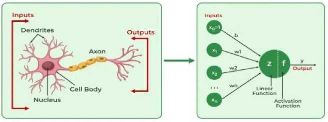
Fig.1. Biological neuron to artificial neuron (Image Sourc e[15])

When multiple neurons are linked together, they form layers. In an ANN, there are three essential layers: the input, hidden layers, and the output layer. The input layer receives the raw data input, the hidden layer performs computations and feature transformations, and the output layer produces the final decision or prediction. This structure allows ANNs to handle complex pattern recognition tasks by learning from data in a way that mimics human cognitive processes. Deep learning architectures are characterized by their depth, which is the number of layers they contain.

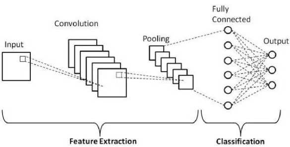
Fig.2. Outline of CNN (Image Source [16])

Convolutional Neural Network (CNNs): This specialized class of deep neural networks that are particularly powerful for tasks involving grid-like data, such as images. CNNs have shown remarkable success in areas of image recognition, classification, and analysis. CNNs are designed to automatically and adaptively learn spatial hierarchies of features through backpropagation by using multiple building blocks, such as convolutional layers, pooling layers, and fully connected layers. Each layer of a CNN transforms one volume of activations to another through a differentiable function. This design allows CNNs to effectively handle the variability and complexity of image data, making them particularly suitable for the task of image-based classification where the input is an image and the output is a label classifying the image content.

Figure 2 shows the typical architecture of a CNN for image classification which includes several layers that each play a crucial role.

While ANNs are general-purpose networks used for structured data tasks like regression and classification, CNNs are specialized for processing grid-like data, such as images, using convolutional and pooling layers to capture spatial hierarchies effectively etc.

Convolutional Layers: These layers perform a convolution operation that filters the input image to create feature maps that summarize the presence of specific features in the input. The first convolutional layer captures lower-level features such as edges and textures, while deeper layers might identify more complex features like shapes or objects. The convolution operation involves sliding a filter or kernel over the input image and computing the dot product of the filter with the image pixels within its field of view. The convolution operation can be mathematically defined as follows:

F(i,j) = (I * K)(i,j) = Z _m Z _n K(m,n) ■ K(i - m,j - n)                          (3)

where I is the input matrix, К is the filter, and 7 is the output feature map at the position (г, J) and m and n iterate over the filter dimensions.

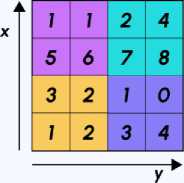
Pooling Layers: This layer also known as subsampling or downsampling typically comes after the convolutional layer. It reduces the spatial dimensions or dimensionality (height and width) of each feature map of the input volume but retains the most important information. This reduction is crucial for decreasing computational complexity and controlling overfitting. Max pooling is one of the most common pooling methods, which involves selecting the maximum element from the region of the feature map covered by the filter. In max pooling, the output for each region of the input is given by:

P(i,j) = max X(i ■ stride + m,j ■ stride + n)

(m,n)eW where W is the area of the window being pooled over, and stride is the step by which the window is slid across the input.

Figure 3 shows an example of max pooling with 2 x 2 filters and a stride 2.

Single depth slice

max pool with 2x2 filters and stride 2

Fig.3. Max-pooling process (Image Source [17])

Fully Connected Layers: After several convolutional and pooling layers, the high-level reasoning in the neural network is done via fully connected layers. Each neuron in these layers is connected to all activations in the previous layer, helping to classify the image based on the features extracted by the convolutional and pooling layers. Their activation can thus be computed with a matrix multiplication followed by a bias offset.

Activation Functions: After each convolution operation, an activation function is applied to introduce non-linear properties to the system, which allows the network to learn more complex patterns. Common activation functions include Rectified Linear Unit (ReLU), Sigmoid and Tanh. ReLU, which is applied after each convolution operation, encourages faster convergence during training by simply thresholding values at zero. Sigmoid and Tanh are functions less used in deep CNNs due to vanishing gradient issues but are still important in the output layers for binary and multiclass classification problems. The ReLU, sigmoid and tanh functions are respectively defined as follows:

f(x) = max(0,x)

^(x) =

i

1+e-x

tanh(x) =

ex

-e

-x

ex+e-x

Softmax Activation Function: This activation function is commonly used in the output layer of neural network models that handle multi-class classification tasks. It converts the raw output scores, known as logits, from the network into probabilities by taking the exponential of each output and then normalizing these values by dividing by the sum of all the exponentials.

Given a vector of raw scores z = [z i ,Z 2 , ...,Z n ], the softmax function a(z) is defined as:

e zi

^(z i ) =                                                          (8)

^i=ie where Zi 6 z is the score for class i, e is the base of the natural logarithm, and the denominator is the sum of all probabilities equaling 1.

This ensures that the output values are in the range [0, 1] and sum to 1, making them interpretable as probabilities. The function is particularly useful when the model needs to classify inputs into multiple categories.

SU^ i ) = 1                               (9)

Loss Functions: The loss function particularly used in classification problems is the cross entropy loss function. This function measures the performance of a classification model whose output is a probability value between 0 and 1. Cross-entropy loss increases as the predicted probability diverges from the actual label. This is mathematically defined as:

L(y c ,f c ) = - Z M=i Y c log(yT)                                     (10)

where j c denotes the true probability or target value for class с, Ус denotes the predicted probability for class c produced by the model, and M the total number of classes.

Backpropagation: This is used for training the neural network. Backpropagation computes the gradient of the loss function with respect to each weight by the chain rule, updating the weights to minimize the loss.

Gradient Descent: A method to update the weights and minimize the loss function. It adjusts the weights incrementally, using the gradient of the loss function.

sl wnew  wold  a gw                                       (11)

where a is the learning rate and w is the weight.

Regularization: L2 Regularization, a regularization technique adds a penalty equal to the sum of the squared values of the weights to the loss function, which helps to keep the weights small and improve the generalization of the model.

Dropout: A simple yet effective regularization technique that prevents overfitting by randomly dropping units (and their connections) from the neural network during training.

• 2.3.    AI Applications in Hospital Waste Management

  In this section, we dive into a comprehensive review of the existing applications pertaining to AI and CNNs in hospital waste management. Firstly, we look at the AI driven solutions tailored for addressing the challenges in hospital waste management, particularly in the resource-constrained developing countries. Then we review the solutions proposed by CNN-based approaches in hospital waste management, particularly waste sorting. We aim to see how AI, and CNNs are revolutionizing sustainable hospital waste management practices. The study by Vu el al. integrates artificial neural network (ANN) waste prediction models with geographic information system (GIS) waste collection route optimization [12]. Using data from Austin, Texas, USA, they predict waste generation rates for recycling and garbage streams in four city sub-areas for 2023. The ANN model yields mean absolute percentage errors ranging from 10.92% to 16.51%. They then create scenarios reflecting potential future changes in waste composition and use GIS tools to determine optimal waste collection routes. Results show significant changes in travel distance, up to 19.9%, compared to non-modified compositions. Also, dual compartment trucks are compared to single compartment trucks, revealing potential travel distance savings between 10.3% and 16.0%, albeit with a slight increase in collection time.

3.    Methodological Approach

• 3.1.    Data Preparation

The methodological framework consists of four primary phases: data preparation, model development, model testing and validation, and model evaluation. Data preparation focuses on gathering, cleaning, augmenting, normalizing, and splitting the data. This is crucial as it ensures the quality of the data, hence having a reliable model’s output. During the model development phase, the architecture of the CNN is built, compiled, and trained using the prepared data. The neural network layers and parameters are set up to learn from the data. Once the model is developed, it goes to the model testing and validation. This test and validation is done using a separate subset of data not seen by the model during the training phase. This is done to assess the generalizability and robustness of the model. The final phase involves applying evaluation metrics to determine the model’s performance, so as to provide insights into the effectiveness of the model in real-world scenarios. Figure 4 visually represents the approach, showing the steps taken for the model’s creation to its evaluation.

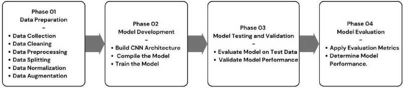
Fig.4. Methodological framework for image classification

To build our hospital waste sorting model, we start with the first step, data preparation. This encompasses several other steps which are crucial for training the CNN model to accurately classify hospital waste. The various steps taken in data preparation, from data collection to data splitting and normalization are as follows.

Data Collection: The data used are RGB images collected from numerous healthcare facilities like hospitals and clinics. They should ensure a diverse representation of waste types. They are gathered and should capture a wide range of hospital waste categories. These color images are represented as three-dimensional matrices known as tensors, with each layer corresponding to a primary color channel (red, green, blue). These matrices encode the intensity values of each color at every pixel location within the image. By processing these matrices, neural networks can extract features and patterns to perform tasks like image classification. This representation facilitates the integration of visual information into the deep learning model’s training process, enabling it to interpret and analyze images effectively.

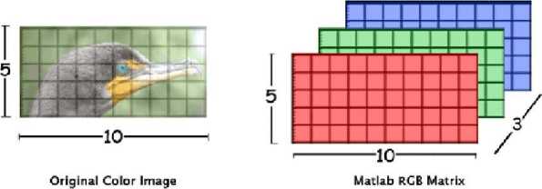
Fig.5. Color image representation and RGB matrix (Image Source [18])

Data Cleaning: The collected data is cleaned to remove samples that could negatively impact the model’s performance, accuracy, and generalizability. This step aligns with the principle of “Garbage in, garbage out”, where poor-quality data leads to poor model performance. Misleading images such as mislabeled samples lead to poor model accuracy, and duplicated samples lead to bias model training and overfitting. Eliminating these samples improves the learning process as it helps the model focus on meaningful patterns, which can lead to more accurate predictions.

Data Prepossessing: Data preprocessing involves several steps, including resizing images, encoding class labels, and structuring the data. All images with suitable file extensions (e.g., .jpg, .png) are resized to a uniform dimension of 224 x 224 pixels to ensure consistency and compatibility across the dataset. Resizing images to a uniform dimension helps reduce the computational burden during training by standardizing the input, allowing the model to process the data more efficiently, improving the model’s training speed. Class labels are encoded using one-hot encoding, which converts categorical data into numerical data for easy interpretation by the model. This ensures that the model can process categorical data without misinterpreting the labels as ordinal. The dataset is also organized into folders, where each folder name corresponds to a specific class label and contains all the relevant images for that class. These preprocessing steps help stabilize the model’s training process, improve learning efficiency, and support better generalization.

Data Splitting: To ensure effective model training and evaluation, the dataset undergoes a crucial step: data splitting. The dataset is split into three subsets: the training, validation, and test set. This separation ensures that the model can be trained on a large set of data (training), parameters can be tuned (validation), and its performance can be evaluated on unseen data (test). Augmentation and shuffling is applied on the training set to increase image variations and randomize the order of samples within each epoch. Two split ratios are used. The first is 70-15-15, 70% for training, 15% for validation, and 15% for testing and the second is 80-10-10, 80% for training, 20% for validation, and 10% for testing.

Data Normalization: In original RGB images, each pixel in the different color channel is represented by values corresponding to their intensity. These intensity values typically range from 0 to 255, where 0 represents no intensity

(black) and 255 represents maximum intensity (full brightness). The pixel values of the images are normalized to a range of [0,1]. This normalization aids in speeding up the convergence of the neural network during training.

The normalization was performed using the formula:

Normalized Pixel Value = OrignaLPixe!—-                                (12)

where / / is the mean of pixel values, and er is the standard deviation of pixel values.

This standardization method centers the data around zero and scales it to have a standard deviation of 1, which can help improve training stability and convergence in machine learning models.

Data Augmentation: To enhance the robustness of the CNN model, data augmentation introduces variations to images using techniques such as random rotation, flipping, shifting, and zooming. These variations simulate how waste items might appear in different orientations, sizes, and positions in real-world scenarios. These variations introduced by data augmentation increase the effective size of the training dataset. This reduces the risk of overfitting, improving the model’s generalization to new, unseen data, especially in cases of limited or imbalanced data. While accuracy offers an initial view of model performance, it may not reflect how well the model handles all classes. A high accuracy may indicate correct classification of majority classes, while the model underperforms on minority classes. To support the accuracy and offer a more complete view of the model’s performance, the F1-score is also considered. The F1-score, being the harmonic mean of precision and recall, offers a balanced measure of performance in situations where class imbalance exists.

• 3.2.    Model Development

In the development of a Convolutional Neural Network (CNN) model, several key processes are involved to construct, optimize, and train the model effectively. These processes include building the CNN architecture, compiling the model with appropriate parameters and optimization algorithms, and training the model on the prepared training dataset. This section outlines the sequential steps involved in developing a CNN model.

CNNs were selected for this task due to their ability to automatically extract hierarchical spatial features from images, eliminating the need for manual feature engineering. This makes them effective for large and complex datasets compared to models such as SVMs or KNNs. Evaluating CNN against these models, CNN was found to be the best choice because of their capacity to learn directly from pixel data, their robustness to variations in image features, and their consistently higher classification performance.

Architecture: The proposed CNN model architecture for classifying hospital waste images is designed with a series of convolutional layers, activation functions, pooling layers, and fully connected layers. This section provides the architectures of the used CNN models.

Model A:

• •    Convolutional Layers: This model is made up of four convolutional layers. Each of these convolutional layers uses the ReLU function to introduce non-linearity, enabling the model to learn complex patterns. The layers progressively increase the number of filters from 32 to 128 of size (3x3), improving the model’s ability to capture finer details within the images.

• •    Pooling Layers: Following each convolutional layer, a max pooling layer with a pool size of (2x2) is used to reduce the spatial dimensions of the output. This step helps in reducing the computational complexity and also helps in extracting dominant features which are invariant to small translations. Here we also have a total of four pooling layers.

• •    Flatten Layers: After the final pooling layer, a flatten layer is used to convert the 2D feature maps into a 1D feature vector. This transformation prepares the data for input into the fully connected layers.

• •    Dropout Layer: A dropout layer is included after the flatten layer. This layer randomly sets a fraction of input units to zero at each update during training time. This helps to prevent overfitting.

• •    Fully Connected Layers: The network includes two fully connected layers. The first has 512 units and uses the ReLU activation, serving as a fully connected layer that processes features extracted from the convolutional layers. The final layer is a dense layer with a softmax activation function. This outputs the probabilities for the number of waste categories.

Model A is built using the split ratio of 70-15-15. Table 2 gives a summary of the provided model’s architecture

Model B:

Model B has the same architecture, optimization algorithm, and parameters as Model A. The only difference between both models is Model B is trained with the split ratio of 80-10-10 while Model A is trained with the split ratio of 70-15-15.

Model C:

Model C is similar to Model A and B, having the same architecture, optimization algorithm, and parameters. The difference between Model C and the other models is it uses the techniques known as k-fold cross-validation.

Table 2. Architecture of the proposed CNN model

Layer	Type	Activation Function	Number of Filters	Filter Size
1	Conv2D	ReLU	32	(3x3)
2	MaxPooling2D	-	-	(2x2)
3	Conv2D	ReLU	64	(3x3)
4	MaxPooling2D	-	-	(2x2)
5	Conv2D	ReLU	128	(3x3)
6	MaxPooling2D	-	-	(2x2)
7	Conv2D	ReLU	128	(3x3)
8	MaxPooling2D	-	-	(2x2)
9	Flatten	-	-	-
10	Dropout	-	-	-
11	Dense	ReLU	512	-
12	Dense	Softmax	num_of_classes	-

K-Fold Cross Validation is a robust method used to evaluate the performance of a machine learning model. This involves dividing the initial training set into K equally sized subsets or folds. Our K in this model is five, so we have our dataset divided into five equal subsets. The model is then trained and validated K times and at each time using a different fold as the validation set. The remaining K-1 folds serve as the training set. The results from each fold are averaged to produce a single estimation of model accuracy. In this particular model with five folds, each training set contains 80% of the initial training set, and each validation set contains 20%.

Validation Sets

Training Sets

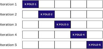
Fig.6. K-fold cross-validation

Given the metric for each fold is Afi, our overall metric ff is:

M ^Z^M i

Optimizer Algorithm: Several optimizer algorithms are often used in image classification using CNN, including Stochastic Gradient Descent (SGD), Root Mean Square Propagation (RMSProp) and Adam. However, this work uses only Adam as the optimizer due to its adaptive learning rate and faster convergence in high-dimensional spaces.

Adam is a popular choice for training deep learning models due to its efficient computation of learning rates for each parameter. Adam combines the advantages of two other extensions of stochastic gradient descent: Adaptive Gradient Algorithm (Adagrad) that maintains a per-parameter learning rate that improves performance on problems with sparse gradients, and Root Mean Square Propagation (RMSProp) that handles non-stationary objectives. The Adam optimizer adjusts the learning rate by estimating the first (mean) and second (uncentered variance) moments of the gradients.

9 t₊₁ = 0 t-4=m- (14)

where &  represents the parameters (weights), if is the learning rate, m t is the bias-corrected first moment estimate, li t is the bias-corrected second moment estimate, and e is a small constant for numerical stability.

• 3.3.    Training

  The models are trained locally on Jupyter Notebook with an Intel(R) Core(TM) i7-6600U CPU @ 2.60GHz, RAM 16GiB computer. The Adam optimizer was used with a learning rate of 0.0001, which was selected based on preliminary tests showing stable convergence at this rate. The models are trained with multiple batch sizes (16, 32, and 64) to evaluate training stability and convergence speed. Smaller batches like 16 yielded more stable training, while a batch size of 64 sometimes led to premature convergence. Each model is trained twice, with epochs set to 30, and 50, striking a balance between training time and model performance while using techniques to prevent overfitting.

For monitoring and improved performance, the two techniques used during the model training are ModelCheckpoint and EarlyStopping.

• •    ModelCheckpoint: This technique is used to save the model’s weight during training, particularly the best performing weights based on a specified metric (usually validation loss or accuracy). The ModelCheckpoint callback is set up to save the model’s weights to a specified file path after each epoch only if the new model has achieved a better performance compared to the previously saved best model. This allows you to later load the best-performing model for inference or further training.

• •    EarlyStopping: Overfitting occurs when a model learns noise and patterns that are specific to the training data but do not generalize well to unseen data. Early stopping is a technique used to prevent overfitting by monitoring the model’s performance on a validation dataset. If the monitored metric (in our case, validation loss) does not improve for a specified number of epochs(patience), training is halted, and the model is restored to the best performing weights observed during training. This helps prevent unnecessary training epochs and ensures that the model does not overfit the training data

• 3.4.    Model Evaluation

At the end of the training phase, the trained model is used to make predictions on the test dataset, which contains data unseen by the trained model. This is done to assess the model’s performance and generalization capabilities. Two important metrics in model testing are test loss, and test accuracy.

• •    Test Accuracy: This metric measures the proportion of correctly classified samples in the testing dataset. It provides insight into the overall performance of the model in terms of its ability to correctly classify unseen examples. Higher values of test accuracy indicate better performance.

• •    Test Loss: This metric represents the average loss (or error) computed across all samples in the testing dataset. It indicates how well the model’s predictions match the true labels in the testing dataset. Lower values of test loss indicate better performance, as they imply that the model’s predictions are closer to the true labels.

4.    Case Study and Validation 4.1.    Context of the Case Study

This study uses the Medical Waste 4.0 Dataset, which consists of hospital waste images collected by Bruno et al[5], accessible via a Github repository. The dataset is a valuable resource for testing computer vision methods for hospital waste sorting. The images were acquired using an OAK-D camera and each sample consists of three images, a RGB image and a stereo pair. The image resolution of the RGB images are 1920 x 1080, and the grayscale 640 x 400. The full dataset is divided into two sub-datasets, named Dataset A and Dataset B. Dataset B was derived from Dataset A, so Dataset A is used as the main dataset for training, validation, and testing the hospital waste classification models.

The Medical Waste 4.0 Dataset was selected for its availability, and diverse representation of hospital waste categories aligned with WHO classification standards. It includes diverse visual representations of hospital waste, captured through RGB and stereo imaging, which simulate real-world conditions in resource-limited hospitals. While some class imbalances exist and the dataset does not fully represent every WHO-defined waste category, it remains one of the most relevant publicly available resources for this task. Medical waste types found in developing countries are generally consistent with those in more developed healthcare systems, further supporting the dataset’s applicability. To address potential biases and improve model generalization, data augmentation techniques were applied during preprocessing. Future validation on additional datasets or in real hospital environments is recommended to further assess model generalizability.

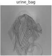
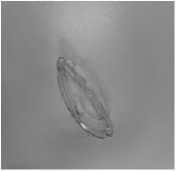
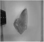
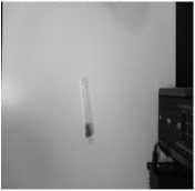
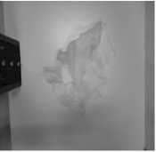
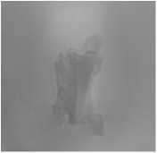
The dataset contains a total of 5520 images, and 13 categories namely: gauze, glove pair latex, glove pair nitrile, glove pair surgery, glove single latex, glove single nitrile, glove single surgery, medical cap, medical glasses, shoe cover single, shoe cover pair, test tube, urine bag.

After thorough data cleaning, duplicate or very similar images in separate categories were discarded. The following pairs: glove single nitrile and glove pair nitrile, glove single latex and glove pair latex, glove single surgery and glove pair surgery, shoe cover single and shoe cover pair were reduced to glove nitrile, glove latex, glove surgery and shoe cover respectively. The final dataset used to develop the model counts a total of 3903 images and a total of 9 categories.

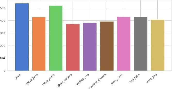
The image distribution, that is the number of files per category is shown in Figure 8. This gives an idea of how balanced or imbalanced the dataset is across the different categories.

medicalcap

medicalglasses

test tube

medical_cap

test tube

gauze

glovejatex

medical_cap

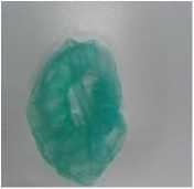
Fig.7. Sample images of the dataset

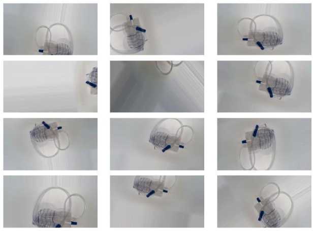
Fig.8. Data augmentation on a training set image

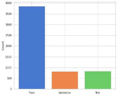
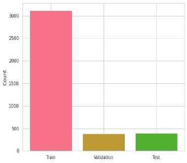
After going through data cleaning, all images were resized to 224 x 224 for size consistency throughout the dataset. Following is data splitting into two different split ratios, 70-15-15 and 8010-10. Figure 9 shows the counts of images in each subset for the two different ratio splits. The data is then normalized after the split, and the following data augmentation techniques were applied on the training set: brightness range ranging from 0.1 to 0.7, rotation range of 90◦, width and height shift range of 0.2, shear range of 0.2, zoom range of 0.2, horizontal and vertical flip set as True.

• 4.2.    Results and Performance Evaluation

In this results and performance section the built models are compared across different metrics, and graphs to distinguish which model performs better. Multiple CNN models, built using various hyperparameters, and optimization algorithms have been evaluated. Table 3 provides a summary of the various model’s development information with the aim to compare their accuracies.

Class

Fig.9. Dataset image distribution of categories

70-15-15 Split Ratio

Fig.10. Data distribution per split ratio

80-10-10 Split Ratio

Accuracy: The performances of CNN Model A and B, discussed in Section 5 are summarized in Table 3. In contrast, Model C, which employs k-fold cross validation is summarized in Table 4. Model A and Model B show a clear differentiation based on training data splits, with Model A being trained with splits of 70-15-15 and Model B on 80-1010.

Table 3. Comparison of CNN models

CNN Model	Optimizer	Batch Size	Epochs	Accuracy
Model A (70-15-15 Split)	Adam	16	30	84.18%
	Adam		50	91.58%
	Adam	32	30	81.65%
	Adam		50	90.74%
	Adam	64	30	74.24%
	Adam		50	78.96%
Model B (80-10-10 Split)	Adam	16	30	89.47%
	Adam		50	84.96%
	Adam	32	30	84.71%
	Adam		50	82.46%
	Adam	64	30	83.46%
	Adam		50	85.46%

Model A, with a more balanced split showed varying levels of accuracy depending on the batch size and number of epochs. The best performance was observed with a batch size of 16 over 50 epochs, achieving an accuracy of 91.58%. However, increasing the batch size constantly led to a drop in accuracy, which shows the sensitivity of the model performance to batch size. Model B, with a larger training set and smaller validation and test set, generally exhibited lower accuracies across most configurations compared to model A. The highest accuracy of model B is 89.47%, which is achieved with a batch size of 16 over 30 epochs. Similar to model A, performances tend to decrease with larger batch sizes.

Compared to Model A where all configurations with 50 epochs performed better than their related configurations with 30 epochs, Model B configurations with 30 generally performed better. Techniques like EarlyStopping and Model Check pointing were used, which permitted all model’s training to stop at its best values once it started overfitting. The comparison of these two models’ results shows the critical impact of data distribution and the training dynamics on the effectiveness of CNN models in classifying complex datasets like medical waste.

Our third model, Model C, was developed using the same architecture and was evaluated using K-fold crossvalidation. In each iteration, the training set was 80% of the dataset and the validation set was 20%. The results of each iteration are summarized in Table 4.

Table 4. K-folds accuracies in model C

CNN Model	K-Folds	Accuracy
Model C	Iteration 1	96.16%
	Iteration 2	96.93%
	Iteration 3	98.85%
	Iteration 4	95.26%
	Iteration 5	98.21%

Model C was trained with a batch size of 16, an Adam optimizer and each iteration consisted of 10 epochs. Their accuracy at each iteration was higher than Model A and Model B with their best configurations. One of the possible reasons could be due to Model C having more training and validation data. The minimum accuracy was seen at Iteration 4 with 95.26% and the maximum accuracy was seen at Iteration 3 with 98.85%. The accuracy of Model C is the average of all five accuracies which gives us 97.08%. Figure 11 is a visual of the accuracies of the various models, and Model C out performs Model A and B.

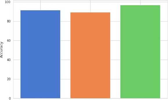
Model A                     Model В                     Model C

Models

Fig.11. Comparison of model A, B, and C accuracies

Precision, Recall, F1-Score Results: The detailed performance metric for the best Model A and Model B reveal some insight in their ability to classify various hospital waste items from our dataset. Based on Model A results found in Table 5, we observe exceptionally high precision, recall, and F1-scores in most categories. This suggests a well-tuned model capable of generalizing effectively across different types of hospital waste. Nevertheless, the categories "gauze" and "glove_latex" have shown low performances, in precision, recall, and consequently F1-score, with the lowest F1-score of 0.76. This may indicate challenges in distinguishing these items from each other due to visual similarities. Another reason could be the way these items appear within the dataset. These edge cases highlight the model’s limitation in distinguishing between visually similar waste items. All other categories in Model A exhibit near-perfect scores, reflecting the model can reliably identify and classify these items with high accuracy.

Model B also shows a good performance across many categories, although generally lower when compared to Model A. Categories like "gauze" and "glove_latex" show lower performances than the other categories, with F1-scores of 0.75 and 0.52 respectively. These results reinforce the classification difficulty posed by these visually similar items.

Model C, which was trained using a larger validation split (20%) and K-fold cross-validation, demonstrates the most robust and consistent performance. The model benefits from improved generalization and higher support across categories. Most precision, recall, and F1-score values exceed 0.90, including significant improvement in distinguishing “gauze” and “glove_latex”, achieving F1-scores of 0.97 and 0.96 respectively. This indicates a strong ability to separate even visually similar classes, suggesting more effective feature extraction and learning under cross-validation.

The use of F1-score as an evaluation metric was particularly important due to the presence of class imbalance in the dataset. F1-score provides a balanced view of precision and recall, offering a more informative measure of model performance than accuracy alone. Overall, Model C stands out as the best-performing model, combining high per-class performance with improved handling of difficult edge cases.

We proceed by taking a look at the confusion matrix of each of these models.

Table 5. Precision, recall, F1-score, and support on best model A

Class	Precision	Accuracy	F1-Score	Support
medical_cap	1.00	1.00	1.00	58.00
glove_nitrile	0.99	1.00	0.99	79.00
shoe_cover	1.00	0.97	0.98	66.00
glove_surgery	0.97	1.00	0.98	57.00
test_tube	0.97	0.98	0.98	65.00
urine_bag	0.86	0.98	0.92	62.00
medical_glasses	0.98	0.83	0.90	60.00
glove_latex	0.70	0.85	0.76	65.00
gauze	0.85	0.68	0.76	82.00

Table 6. Precision, recall, F1-score, and support on best model B

Class	Precision	Accuracy	F1-Score	Support
medical_cap	1.00	1.00	1.00	39.00
glove_nitrile	0.97	1.00	0.99	38.00
shoe_cover	1.00	0.93	0.96	44.00
glove_surgery	0.93	1.00	0.96	40.00
test_tube	0.98	0.95	0.96	42.00
urine_bag	0.95	0.95	0.95	44.00
medical_glasses	0.96	0.94	0.95	53.00
glove_latex	0.65	0.89	0.75	55.00
gauze	0.72	0.41	0.52	44.00

Table 7. Precision, recall, F1-score, and support on best model C

Class	Precision	Accuracy	F1-Score	Support
medical_cap	1.00	1.00	1.00	83.00
glove_nitrile	1.00	1.00	1.00	83.00
shoe_cover	1.00	1.00	1.00	73.00
glove_surgery	0.99	1.00	1.00	113.00
test_tube	1.00	0.96	0.98	75.00
urine_bag	0.97	0.99	0.98	88.00
medical_glasses	0.97	0.97	0.97	92.00
glove_latex	0.92	1.00	0.96	83.00
gauze	1.00	0.92	0.96	90.00

Confusion Matrix: The confusion matrix of each model offers detailed insights into the classification performance of each model across different categories of hospital waste. The diagonals in this confusion matrix represent correctly classified instances for each class, that is True Positives (TP).

Model A shows very good classification with a very high number of True Positives across the different categories. Categories like "glove_nitrile", "glove_surgery", and "medical_cap" have the highest true positive rates indicating effective recognition and classification. Other categories have maximum one or two misclassifications, which is still very good but the categories "medical_glasses", "gauze" and "glove_latex" show more misclassifications than others. The category "gauze" and "glove_latex" show the lowest TP, that is the highest misclassification. There are occasional instances where "medical_glasses" are classified as "urine_bag" but "urine_bag" is only misclassified in one instance as

"glove_nitrile".

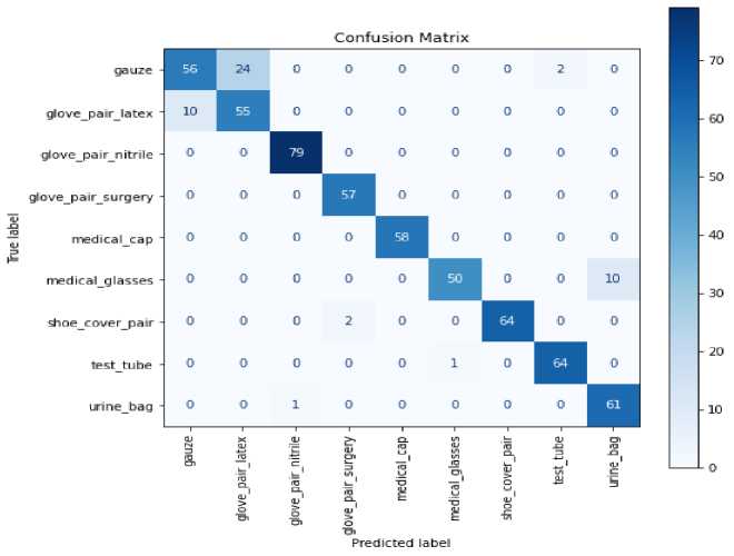
Fig.12. Confusion matrix - best A

Model B, generally shows a good performance as well, particularly in the categories "glove_nitrile", "glove_surgery", "medical_glasses" and "medical_cap" which still have a TP rate of 100%. There are few misclassifications in other categories except "gauze" and "glove_latex" which have a higher number of misclassifications despite having fewer test samples compared to Model A.

While Model A tends to maintain a more balanced performance across most categories, Model C shows a near perfect classification of most hospital waste categories even though Model A and B struggled with categories "gauze" and "glove_latex". Though a higher number of samples to test it still shows better performance than Model A and B. This suggests that a larger training and validation set is crucial for achieving a good performance.

The categories our model has faced a lot of challenges to properly classify are "gauze" and "glove_latex". Having a visual of some images from these two categories would give us an insight of why challenges are faced in classifying those two categories.

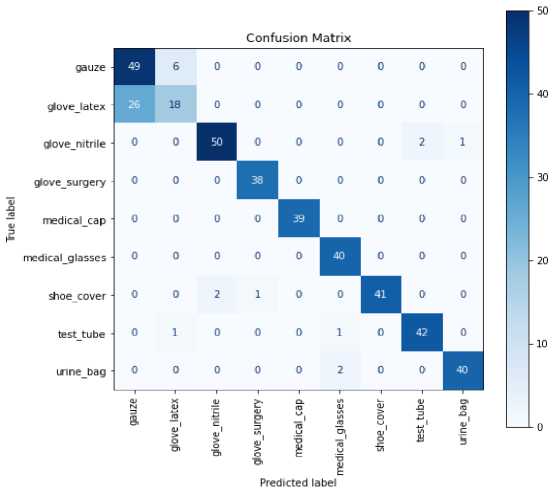
Fig.13. Confusion matrix - best B

Looking at the images present in the category of "gauze" and "glove_latex", we could have an understanding of why they face difficulties in properly classifying them as they look alike.

Model C has shown to be a robust model with robust feature extraction as it was able to classify the "gauze" and "glove_latex" images despite their visual similarities.

ф

Confusion Matrix gauze glove_latex glove_nitrile glove_surgery medicalcap medicalglasses shoe cover test tube unne_bag

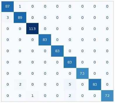
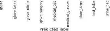
Fig.14. Confusion matrix - best C

Learning Curve: Model A shows a steady increase in training accuracy over 30 epochs, reaching a peak and maintaining stability, which indicates effective learning without significant overfitting. However the validation accuracy shows slight fluctuations but remains close to the training curve which is a good sign of good generalization. The loss plot shows a sharp initial decrease, stabilizing as epochs progress. There are also periodic spikes in validation loss indicating moments of learning adjustments.

Model B shows a more rapid convergence in accuracy, achieving higher validation accuracy peaks compared to Model A. This suggests that the increased training data proportion impacts the model’s ability to generalize from fewer epochs. However, the loss plot for Model B shows higher variability, especially in validation loss, which could indicate potential overfitting despite higher accuracy scores.

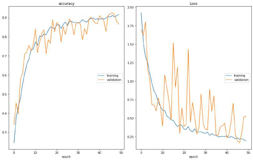
Fig.15. Learning curve - best A

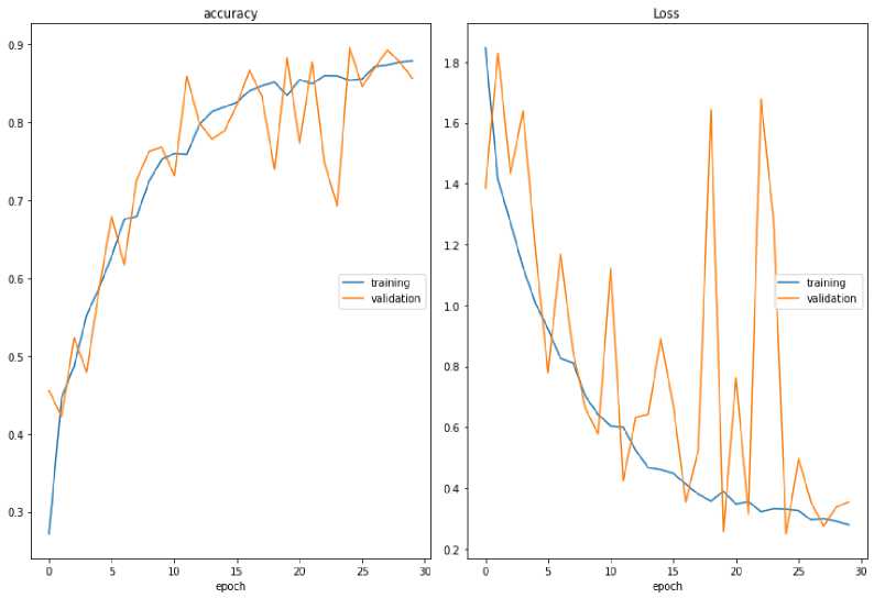
Fig.16. Learning curve - best B

Model C shows a steady increase over the epochs, indicating that the model is learning effectively from the training data. The validation accuracy improves as well, though showing more variability. Both curves exceed 0.95, suggesting the model is not overfitting and has good generalization performance.

The training loss decreases consistently, indicating the model is reducing its error on the training data. The validation loss follows a similar pattern. The final loss values are low, below 0.2. This indicates the model has learned effectively and is performing well on both the training and validation sets.

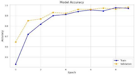
Fig.17. Accuracy learning curve of model C

The evaluation of our models in this study shows the significant potential of CNNs in improving hospital waste management. While Model C demonstrated superior performance in most configurations, with an accuracy of 97.08%, the other models showcased the critical role of handling model parameters in achieving high classifications. This research paves the way for future developments in AI applications for sustainable waste management, emphasizing the need for further improvements in model robustness. This study’s insights are particularly very important for advancing hospital waste management solutions in developing countries and improving public health and environmental protection.

• 4.3.    Discussion and Perspective

5.    Conclusions

The findings of this study highlight the practical viability and strong performance of AI-based approaches particularly CNNs in classifying and sorting hospital waste. With an accuracy of 97.08% and high F1 -scores, the proposed model demonstrates strong potential for improving waste management efficiency, reducing dependency on manual sorting, and minimizing human exposure to hazardous materials. These results validate the applicability of deep learning techniques in addressing real-world environmental and health challenges, especially in settings where traditional waste management methods are inadequate or unsafe.

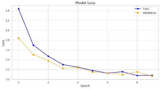
Fig.18. Loss learning curve of model C

Despite the promising results, the implementation of such AI-based systems in developing countries remains constrained by several challenges. These include limited access to digital infrastructure, inconsistent data quality, lack of skilled personnel, and the high cost of deploying and maintaining intelligent systems. In addition, AI applications in healthcare and environmental sectors raise ethical concerns related to data privacy, fairness, and accountability. Without addressing these limitations, there is a risk that such technologies may fail to deliver meaningful impact or could even exacerbate existing inequalities in healthcare service delivery and waste management practices.

Advancing toward sustainable adoption of AI in healthcare waste management requires a comprehensive, multipronged approach. Key components include the development of well-defined regulatory frameworks to guide AI integration, the promotion of public-private partnerships to harness financial and technical resources, and the creation of context-specific solutions tailored to the operational realities of local hospital settings. Strengthening local capacity through education and skill development is vital to ensure the effective operation, maintenance, and scalability of these technologies. Additionally, the phased rollout of pilot initiatives, with active engagement from both communities and institutions, can provide valuable insights for refining AI models and evaluating their long-term viability. With strategic planning and inclusive governance, AI technologies can significantly enhance the safety, efficiency, and sustainability of healthcare waste management systems throughout the Global South.

This work focused on harnessing the capabilities of Convolutional Neural Networks (CNNs) to improve the classification and segregation of hospital waste. This is a crucial aspect of healthcare management that impacts both public and environmental health, especially in resource-constrained and developing countries. By leveraging deep learning techniques, we aimed to develop a model that could accurately identify and categorize various types of hospital waste from images (visual data). Our objective was to design and test CNN models that could enhance the efficiency and accuracy of hospital waste management systems. We sought to evaluate these models across different configurations and training splits to understand their performance dynamics and identify optimal conditions for effective waste classification. Although this study was based on a specific dataset, future validation on external or real-world datasets is necessary to ensure robustness across diverse hospital environments. The results demonstrated that our CNN models, particularly Model C which used k-fold cross validation, achieved an accuracy of 97.08% in classifying medical waste types. Due to class imbalance present in certain categories, the F1-score was analyzed to provide a more balanced evaluation of the model’s performance. Model C recorded excellent F1 scores ranging from 0.96 to 1 across various classes, reinforcing its status as the best-performing model, reflecting the model’s true general performance. The performance disparities between the categories "gauze" and "glove_latex" suggested the need for more robust feature extraction techniques or enhancing datasets that have better representations of these various categories. The performance evaluation revealed that specific model parameters and training conditions significantly influenced the models’ effectiveness. This shows the importance of robust dataset preparation in developing practical AI applications for hospital waste management. Scalability to larger datasets and adaptability to more complex hospital waste scenarios remain critical next steps. Real-world implementation challenges such as infrastructure limitations, equipment availability, and staff training must also be considered when deploying such AI systems in hospital environments.

All the Declarations and StatementsAuthors Contributions Statement

Teddy Ako Eyonganyoh - Methodology, Data Curation, Software, Validation, Formal Analysis, Visualization, Writing - Original Draft: Designed the methodological framework, performed data cleaning and preprocessing, implemented the research model, trained and validated models, conducted comparative performance evaluation using standard evaluation metrics, analyzed experimental results, prepared performance visualizations, drafted the initial manuscript, and conducted literature review.

Justin Moskolaï Ngossaha - Conceptualization, Data Curation, Supervision: Proposed the research topic and ideas, provided the dataset, constructed the overall framework, and supervised project execution.

All authors have read and agreed to the published version of the manuscript.

Conflict of Interest Statement

The authors declare no conflicts of interest.

Funding Declaration

None

Data Availability Statement

This study analyzed publicly available datasets. The datasets can be found here: , accessed on Mar. 25, 2026.

Ethical Declarations

Not applicable. This study does not involve human or animal subjects.

Acknowledgements

The authors express their deepest gratitude to the African Institute for Mathematical Sciences (AIMS) Cameroon for providing the essential academic environment, facilities, and resources that made this research possible. We sincerely thank the journal reviewers and experts for their professional evaluation and valuable recommendations, which have contributed to improving the quality of the experiment and the reliability of its results.

Declaration of Generative AI in Scholarly Writing

The authors used AI-assisted tools to strengthen the language and readability of the manuscript. All outputs were reviewed and edited with human oversight, and the authors take full responsibility for the final content.

Abbreviations

The following abbreviations are used in this manuscript:

AI - Artificial Intelligence

ANN - Artificial Neural Network

CNN - Convolutional Neural Network

DT - Decision Tree

GIS - Geographic Information System

KNN - K-Nearest Neighbors

ReLU - Rectified Linear Unit

RGB - Red, Green, Blue

RMSProp - Root Mean Square Propagation

SGD - Stochastic Gradient Descent

SVM - Support Vector Machine

WHO - World Health Organization