Algorithm for processing the results of calculations for determining the body of optimal parameters in the weighted finite element method

Mathematical models in the form of boundary value problems with a singularity play an essential role in fracture mechanics. The Lam´e system or biharmonic equation is used for the crack problem or the elasticity problem in a domain with a broken in the boundary. In domains with reentrant corners at the boundary, the Stokes problem or the system of Maxwell’s equations are used in hydrodynamics or electrodynamics. Numerical methods for boundary value problems with a singularity were actively developed recently. For instance, the different finite element methods (FEM) were constructed for solving of the crack problem; among them we note smoothed FEM [1, 2], meshless/meshfree methods [3, 4], Extended FEM (XFEM) [5–7], field-enriched FEM [8, 9], FEM on mesh with compression [10,11].

We proposed to define the solution to boundary value problems with strong and corner singularities as an R ν -generalized solution [12–15]. The presence of the weight function in the integral identity of the definition of the R _ν -generalized solution made it possible to create a numerical method without loss of accuracy. The singularity of the solution does not affect the rate of convergence of the approximate solution to the exact one. The weighted finite element method (WFEM) for the boundary value problems of the second-order elliptic equations [16], to time harmonic Maxwell equations with strong singularity [17] and Stokes problem with singularity in a 2D non-convex polygonal domain with one reentrant corner [18–20], and the crack problem in the theory of elasticity [21, 22] was developed.

Three control parameters ν, ν ^∗ , δ must be set to find an approximate solution by the weighted finite element method. An algorithm for determining the body of optimal parameters (BOP) for the crack problem was presented in [22]. An approximate solution is found with an error that does not deviate much from the best error in the norm of the weighted Sobolev space or the weighted energy norm when choosing control parameters from BOP. The algorithm for finding the BOP is based on processing the results of calculations of a series of typical problems. This approach is substantiated by the uniform representation of the asymptotic expansion of the solution to any of the crack problem and by the established interval for the parameter ν from the theorem on the existence and uniqueness of the solution.

In this paper, we present an algorithm for processing the results of calculations and determining the BOP for the Lam´e system in a domain with a reentrant corner from π to 2n at the boundary.

1.    Rν -Generalized Solution and Weighted Finite Element Method

We consider a boundary value problem for the Lam´e system with constant coefficients A and ц with respect to the displacement field u = (u 1 ,u ₂ ):

- (2 div(^e(u)) + v (A div u)) = f, x G Q,                    (1)

u = q , x G dQ.                                (2)

Here e(u) is the strain tensor, f is a distributed body force, Q is a bounded non-convex polygonal domain with the boundary dQ containing one reentrant corner such that its vertex is located in the origin O(0,0).

Let Q ‘ = { x G Q : (x 2 + x 2 ) ^1/2 <  5 ^ 1 } be the ^-neighborhood of the point O(0,0) in Q. We introduce a weight function p(x) that coincides in Q with the distance to the origin, i.e. p(x) = (x 1 + x 2 ) ^1/2 for x G Q ‘ , and equals to 5 for x G Q \ Q ‘ .

Denote by W ₂1 _a (Q,5) the set of functions satisfying the following conditions:

• a)    | D ^m u(x) | <  c 1 (5 \ p(x)) ^a+m for x G Q , where m = 0,1, the constants c 1 > 1 is independent of m;

• b)    ||u(x) ||_L 2 _a (Q \ Q') >  c ₂ , where c ₂ = const; with the squared norm

Н^ад = E p(x) | D m u(x) iH L ₂ (Q) ,

| m |< 1

where m = (m 1 ,m ₂ ) and | m | = m 1 + m ₂ , and a is a real nonnegative number.

We use the notation W 2 _a (Q, 5) for the corresponding set of vector functions.

Define R _ν -generalized solution to problem (1), (2) as a function u _ν from the set W 2 _a (Q, 5) that satisfies the boundary value conditions on dQ and satisfies the following integral identity:

a(u _v , v) = l(v) for all v = (v 1 ; v ₂ ) G W 1, _v (Q,5).

Here a(u, v) = J (2^(u)) : e(p ^2v v) + A div u div (p ^2v v))dx, l(v) = J p² f • vdx. Q                                                Q

The weighted finite element method for finding an approximate R _ν -generalized solution to problem (1), (2) was constructed in [23]. Here we briefly describe construction of the WFEM.

We perform a quasi-uniform triangulation of the domain Q. Let K be the union of all the triangles K i , i = 1,... ,n; h be the maximal length of the sides of the triangles. We refer to h as a mesh step. The vertices P i , i = 1,..., M of the triangles K are nodes of the triangulation, {P M } = {P 1 ,..., P M } and the point O G P M . Let P = {P k } k=N be the set of internal triangulation nodes.

To each node P i G P we assign the weighted function

^i = pv*(x)^i, i = 1,... ,N, where ϕi is a linear function on each triangle K equal to 1 at the node Pi and zero at all the other nodes, ν∗ is a real number.

We introduce the weighted vector basis { ^ _k (x) } k=1N , where

^ k ^(x) = |

(^i(x), 0),k = 2i - 1, (0,^i (x)),k = 2i, i = 1,...,N.

Denote by V h the linear span { ^ _k (x) } _k =1N . In V h we consider the subset V ^h = { v G V h : v(P i ) = 0,P i G dQ } .

In the space V h , a function u h is called an approximate R _v -generalized solution of problem (1), (2) by the weighted finite element method if u h satisfies boundary value condition (2) for the mesh nodes P i G dQ and the integral identity

a(u h , v h ) = l( v h ) holds for all v h G V h .

An approximate solution is found in the form

2N

Uh = ^dk ^k (x)’ k=1

where d k = p ^{- v} * (P [(k₊i)/2] )c k , C k = ( U iH P !^ ¹ )/ ² ] ]’ k _ 2i    ¹ , i = 1,. . . , N, [(k + 1)/2]

I Uv,2(P[(k+1)/2]),k = 2i is integer part of the number (k + 1)/2.

In contrast to the classical FEM, the weighted finite element method allows to find a solution to problem (1), (2) with an accuracy of O(h).

2.    Algorithm for Determining Body of Optimal Parameters

We need to set the parameters ν, ν ^∗ , δ to calculate the approximate R _ν -generalized solution to boundary value problem (1), (2) by the weighted finite element method with the smallest error. There exist no theoretical methods for determining the optimal parameters v, v * , 5, so we determine these parameters experimentally for different corners w (п C w C 2п). We use data on the permissible intervals of the parameters v and v * . The admissible values of the parameter ν are in the half-interval, which is established in the existence and uniqueness theorem of the R _ν -generalized solution [13]. The values of the parameter v * are determined from the interval [0, 0,49] based on the asymptotic of the solution to problem (1), (2) [24].

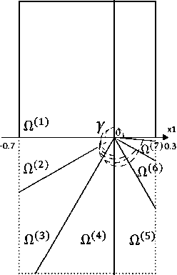
The algorithm for determining the BOP is given in [22]. We consider two model problems (1), (2) in the domains Q ⁽ⁱ⁾ with reentrant corners w i = п + ⁿ (i — 1),i = 1,..., 7 (see Fig. 1).

Problem (A _i )

K i 1   .п    /6\ Г A . ₂ /6А]

u ¹ = 7?Г "i ^cosW P ^— • ■ ^{+ sln} ШJ’

Kt 1         /е\ r a „ /»\i u2 = 7TSr"i ВШЫ [2 — A7^ — cos Ы ]'

Lame coefficients are A = 576, 923,7 = 384, 615, and the stress intensity factor is K I = 1, 611.

Problem (B _i )

u 1 =

K i 1 n.

--■= r “ cos

^ y2n

(d1

-

λ

A + p

+ sin ² (0] + r ² ,

K I  1    n_    (e

= T Ж “i ^sin (2) [²

λ

A + ^

2 ©I

The solution to problem (A i ), i = 1,..., 7 is singular. The solution to problem (B i ), i = 1,..., 7 contains singular and regular components.

In Q(i) ,i =    1,..., 7, we construct the quasiuniform meshes Hj (j   =   1,..., 6) with the step h = 0, 062, 0, 031, 0, 015, 0, 0077,0, 0038, 0, 0019. For each problem (Ai), (Bi) and each mesh Hj we determine three parameters ν, ν∗ , δ for which the relative error in the weighted Sobolev norm is the smallest. We form the sets (Аг,Н3) НАК) АЛК) (HBiK) НАК) of parameters T^      , T2      , T3      , T1      , T2      ,

TН) and Tij = T(AHj) Q TВН),k = 1, 2, 3, at which 3                 k         k             k the relative errors differed from the best error by no more than 5% (6.5%), 10% and 15%. For each mesh Hj the body of optimal parameters is Tj = Qi=1 T^j, k = 1, 2, 3.

+ r ² , i = 1,..., 7.

_lx2 1

-1

Fig. 1. Domains Q(i), i = 1,..., 7

3.    Algorithm for Processing Calculation Results. BOP Visualization

An approximate solution to problem (1), (2) for given initial data (coefficients, righthand sides of the equation and boundary value conditions, parameters h, ν, ν ^∗ , δ) was found using the program “Proba-IV” [25]. An algorithm and a computer program for processing the results of calculations of a large series of problems and determining the BOP were developed. The created program allows:

• •    to define the sets T^ j = T ^{( A,H j} ) Q T ^{( Bl,H j} ) , k = 1, 2, 3, for the fixed mesh Hj- (j = 1,..., 6) and the domain Q ⁽ⁱ⁾ , i = 1,..., 7;

• •    to determine the BOP T j = Q i=1 T^j , k = 1, 2, 3, for each mesh H j (j = 1,..., 6) and the set of domains Q ⁽ⁱ⁾ , i = 1,..., 7;

• •    to visualize the sets T ^i,j and the BOP;

• •    to create tables with intervals of control parameters included in a BOP.

The calculation results of problems (A _i ) or (B _i ) on the mesh H j for fixed parameters δ , ν , ν ^∗ were used as input data:

• •    an identifier of the calculated problem;

• •    a mesh step label;

• •    values of control parameters;

• •    values of the exact solution in norms of the spaces L ₂ (Q), W^ v (Q), E v (Q) and in a seminorm W^ v (Q);

• •    values of the errors for an approximate solution in norms of the spaces L ₂ (Q), W^v (Q), E v (Q) and in a seminorm W ₂1 _v (Q);

• •    values of the relative errors for an approximate solution in norms of the spaces L ₂ (Q), W ₂¹v (Q), E v (Q) and in a seminorm W 1v (Q);

• •    values of the approximate solution in norms of the spaces L ₂ (Q), W^ v (Q), E v (Q) and in a seminorm W ₂1 _v (Q).

3.1555894824096118733702809e-02 0.030936 0.9 0.1

First, we form a text file from the input data containing the value of the norm of the relative error and the corresponding values of the parameters 5, v, v * . For example, when analyzing the error in the space norm W ^v (Q) the data sample has the following form:

Fig. 2 . Example of a sample data

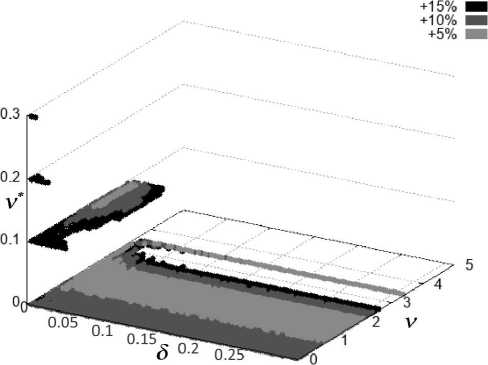
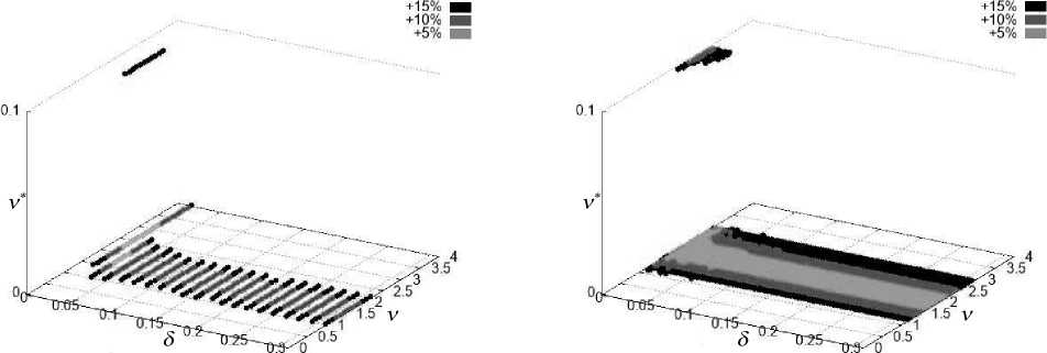
Further, for all parameters 5, v, v * from the specified ranges, a row with the smallest norm of the relative error is selected and an array of rows is formed in ascending order of error. Out of the entire set of rows, we select three subsets T ⁽ A i H ) , T ^{( A} i H ³ ) , T A i H j ) or T B i ^{H j} ) , T ^{( B} i ^{,H j} ) , T ^{( B} i ^{H j} ) at which the relative errors differed from the best error by no more than 5%, 10% and 15% (see, for example, Fig. 3). Then, the sets T ij = T (A i H ³ ) П T ^{( B i} H³ ) , k = 1, 2, 3 are determined.

kk k

b)

+15% ■

+10% ■

+5% ■

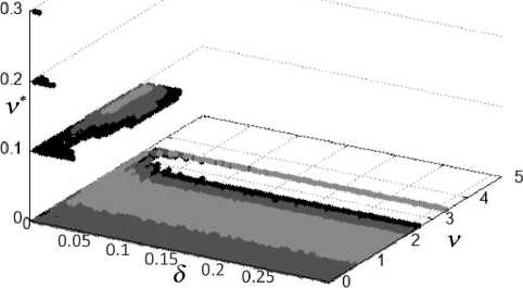
Fig. 3 . (3а) the sets T A) , T ₂ ⁽ A ^{5 )} , T ₃ ⁽ A ^{5 )} ; (3b) the sets T (B 5 , T ₂ ⁽ B ^{5 )} , T ₃ ⁽ B ⁵ ) ; (3c) the sets T j ,j = 1, 2, 3 for the mesh with a step h = 0, 0038

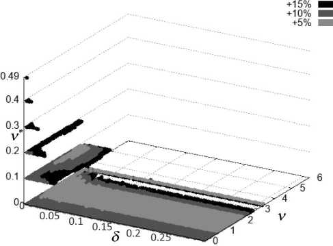
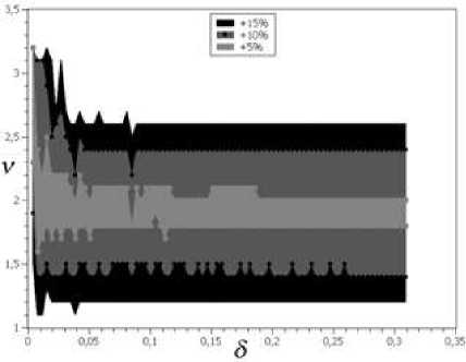
We say that the BOP is a set of parameters 5, v, v * which is simultaneously included in all T^ j in the domains Q ⁽ⁱ⁾ , i = 1,..., 7 for a fixed mesh H j (j = 1,..., 6), i.e. T j = n i=i T k'j , k = 1, 2, 3 (see, for example, Fig. 4).

At the next step, the program, by exhaustive search and comparison of the corresponding parameters, determines the BOP. In some cases, it is possible to determine the BOP not for all domains Q ⁽ⁱ⁾ , i = 1,..., 7 but for separate groups, for example, for problems in domains with reentrant corners {180 ° , 210 ° , 240 ° } or {270 ° , 300 ° , 330 ° , 360 ° }.

а)                                                       б)

Fig. 4 . The body of optimal parameters for the mesh with steps h = 0, 015 (4a) and h = 0, 0019 (4b) together for all domains Q ⁽ⁱ⁾ , i = 1,..., 7

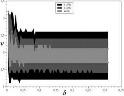
In addition, we determine the BOP at which the deviation of the relative error from the best one does not exceed 5% and 6% (see, for example, Fig. 5). This indicates the sustainability of the process. The error changes insignificantly with a small deviation in the choice of parameters from the best parameters.

a)

Fig. 5 . Parameter values at which the deviation of the relative error from the best one does not exceed 5% and 6% for all domains Q ⁽ⁱ⁾ , i = 1,..., 7 on the mesh with a step h = 0, 0038

b)

Various sets of parameters and the BOP visualization was carried out using the “gnuplot” program [26]. The input text file contained the values of parameters 5, v , v * on each line. These parameters determined the coordinates of a point in three-dimensional space. The error ranges were indicated in the executive file for correct visualization.

• •    The parameter v * was sequentially assigned the values 0, 0, 0,1, 0, 2, 0, 3, 0,4, 0,49.

• •    For each value of v * and 5 = h, 2h, 3h, ... an interval of parameters was chosen for which the approximate solution error norm deviated from the minimum error by no more than a given limit value.

• •    For each value of v * intervals of 5 were determined with the same intervals of v.

As a result, the table was formed (see, for example, Table).

The choice of the optimal parameters for the weighted finite element method provides the creation of codes for finding an approximate solution with high accuracy for problems of elasticity theory with a corner singularity.

Table

Table sample

Percent of error	δ	ν	ν ∗
5%	1h-5h	0,6...1,4	0
	1h	0,7...3,1	0,1
6.5%	1h-5h	0,5...1,5	0
	1h	0,5...3,3	0,1
10%	1h-5h	0,1...1,8	0
	1h	0...3,8	0,1
	1h	0,4...2,9	0,2
15%	1h-5h	0...2,9	0
	1h	0...4,3	0,1
	1h	0...3,9	0,2

Acknowledgments. The reported study was supported by the Russian Science

Foundation, project No. 21-11-00039,