An EfficientNetB3 Approach for Retinal Disease Classification with XAI and Online Interface

In the past few years, the application of deep learning (DL) models to interpreting medical imaging pictures has grown a lot. These models are particularly useful for diagnosing and treating a wide range of disorders. This is because deep learning has made computer vision (CV) development possible, which has never been seen before in the identification and categorization of diseases. But there is still one problem: medical practitioners will probably require help interpreting the projections from these algorithms since they are hard to understand. Eye detection is a key part of computer vision that might be used for surveillance, biometrics, medical, and human-computer interaction. Convolutional neural networks have been the best way to find objects for a long time. They have changed computer vision with deep learning. Recently, a lot of people have been interested in novel transformer designs because they can describe complex connections between input data using self-attention techniques. By effectively distinguishing eye characteristics and developing effective representations, these models have reached the highest level of performance in a number of CV tasks, including eye recognition. The good results are gratifying, but the fact that conventional deep learning models are hard to understand might lead to wrong diagnoses and treatment plans that hurt patients. The World Health Organization, or WHO, reports that a lot of individuals around the world have trouble seeing. Progressive macular degeneration, diabetic retinal degeneration, glaucoma, and cataracts are the most common ones. Because of population expansion, aging, and rising diabetes rates, it is thought that all of these eye illnesses will become more common over the world. This study intends to solve the problem of interpretability by adding Explainable AI (XAI) methods to a novel system for finding and classifying eye diseases. XAI gives medical professionals a better grasp of the DL model’s predictions and helps them trust them. The suggested strategy involves training the model on vast sets of medical images so that it can accurately find a wide range of eye illnesses. To get the best accuracy, this is also done via methods like data augmentation and careful parameter tuning. Using XAI methods makes the model easier to grasp, which makes it easier for medical professionals to figure out why it made the forecast. The research shows that this method is higher than traditional models regarding accuracy, interpretability, and resilience. This is a new contribution to the area of medical imaging. The suggested model and XAI approaches together can make a big difference in medical imaging, which will help make healthcare policy more efficient and successful. This technique is being developed since healthcare is relying more and more on medical imaging and there is a need for models of illness diagnosis that are both accurate and easy to understand. This study helps move medical image analysis forward by getting around the problems with traditional deep learning models. It also lays the groundwork for future research into how to use XAI approaches in healthcare systems. The results show that better early diagnosis of eye illnesses might improve patients’ outcomes and lower the number of people who lose their eyesight throughout the world.

This research primarily aims to enhance the diagnosis and interpretation of eye diseases using deep learning and Explain- able AI methods. The specific objectives of the study are:

• •    To develop a deep learning model that accurately detects and classifies eye diseases using a large set of medical imaging data.

• •    To integrate XAI techniques (such as SHAP and LIME) into the model to improve its interpretability, helping medical practitioners understand the rationale behind the predictions.

• •    To evaluate the effectiveness of the proposed approach in terms of accuracy, interpretability, and robustness when applied to real-world medical data.

2.    Literature Review 3.    Materials and Methodology 3.1.    Dataset Description

Following the introduction, Section 2 provides a detailed literature review on recent works performed in the areas of medical image processing and eye disease classification, which describe existing methodologies and gaps in the literature. Methods: Section 3 describes the methods used in this study, including the design of the deep learning model, integration of Explainable AI (XAI) techniques, and data augmentation strategies to enhance performance and interpretability. The implementation and experimental setup are described in Section 4, including the hardware configuration, the model training and testing procedures, and the interpretation of the results. Performance evaluations and comparison with existing models are given in section 5, and discussion of the results is this section. Last section, that is section 6 finalizes the research paper by reviewing the main findings and discussing the future work in eye disease detection and use of XAI for health care improvement.

Mishra et al. Machine learning was proposed as a means of early detection of various disorders such as diabetic retinopathy, glaucoma and cataracts in the eyes [1]. T heir CNN based model was 91% accurate in classifying eye images. To improve health-assistive usability, they further used XAI methods and developed a user-friendly intuitive GUI for real-time diagnostics. Sharma Gupta et al. [2] I n another study different from the above, a deep learning technique based on VGG19 model was utilised to classify healthy and unhealthy retinal images of the eye. The technique was geared toward eye diseases such as diabetic retinopathy, glaucoma and cataracts. They achieved an accuracy of 95% using a pre-trained CNN. Transfer learning is a viable method for improving early detection in medical imaging, and especially in the field of ophthalmology, researchers reported. Aya A. Abd El-Khalek et al. [3] U sing fundus images, a computer-aided diagnostic (CAD) system for some stages of classifying age-related macular degeneration (AMD) was designed. In local and global texture analysis, GLCM and GLRLM feature extraction methods were used in the proposed system. Photos were then classified into the appropriate category (geographic atrophy (GA), intermediate AMD, wet AMD or normal) using a maximum weighted majority voting method. It did so with 96.85% accuracy. This work demonstrated that the fused dataset of handwritten features with ensemble models could assist physicians in the rapid and precise diagnosis of AMD. Nouf Badah et al. An automated approach to glaucoma detection using classical machine learning and deep learning methods was presented in [4] . They evaluated the outputs of many popular classifiers, including SVM, KNN, NB, MLP, DT, and RF, in order to find the optimum method for reliable diagnosis. The CNN outperformed other models, with an accuracy exceeding 84% in their results. RF and MLP also performed similarly, achieving an accuracy of 77%. In this work, it is demonstrated the effectiveness of Deep learning methods, especially CNNs, in detecting eye diseases from medical image databases. Gao et al. Machine-based Cataract Detection for Bulk Screening and Grading The solution for detecting cataract with machine based system is proposed by Guo et al. [5] a nd it was a novel idea for the bulk screening and grading of the cataract. A strategy using enhanced texture features and LDA achieved a 84.8% success rate on a clinical database. Yang et al. Using a top-bottom hat modification to emphasize the differences between foreground and background, a three-step strategy for effectively automatically discovering cataract was developed. They used both brightness and texture as attributes and BBNN for classification of cataracts into mild, medium, and severe classes. Guo et al. Wiwik Fuadah et al. [6]bu ilt a Computer-Aided Classification System of Cataract with Feature Extractions Based on fundus images, Wavelet Transform and sketch-based methods. They achieved 90.9% accuracy by using wavelet transform-based characteristics. However, KNN was able to distinguish normal from cataract cases with 94.5% accuracy, but it required a different methodology using statistical texture classification and human segmentation. Yang et al. [7] then p roposed an ensemble learning model to detect and score cataracts. Cataracts were detected with an accuracy of 93.2% and graded with 84.5% accuracy using this method. Caixinha et al. A method that allows for living diagnostic of cataracts using ultrasonic imaging and machine-learning algorithms [8]. T hey evaluated different classifiers (SVM, CatBoost, etc.) It is infallible though costly and invasive. An SVM classifier was used to classify fundus images in a different study and the model achieved an accuracy of 93.33% in detecting the severity of cataracts. A smartphone-based app for self-screening for cataracts was also developed that used texture analysis and was expected to be 85% accurate. Jagadale et al. Hough circle detection was used to center and diameter of lens [9]. With the help of an SVM classifier they successfully found cataract with a 90.25% accuracy. Sigit et al. [13] employed a single-layer perceptron; They found a way to detect catar999act using Android smartphones with 85% accuracy. An advanced approach employs hierarchical feature extraction and neural networks to simplify cataract grading. Detection [10] a nd grading exactitude were 94.83% and 85.98%. Cataracts have been commonly detected by DL methods recently. Gao et al. A DL-driven approach for rating nuclear cataracts. Another study recommended a shallow CNN for cataract detection with an accuracy of 93.52% Ran et al. A 90.69% accurate six-level cataract grading method was suggested by [11] b ased on combining Random Forests and Deep CNNs. An automated cataract detection was developed using transfer learning on a CNN (accuracy: 92.91%). Jun et al. Their paper [12] described a cataract grading system that employed a Tournament-based RankedCNN and binaryCNN model. Hossain et al. proposed an automated detection method based on DCNNs using ResNet and achieved an accuracy of 95.77%. Recently, Zhang et al. In ultrasound images, an attention-based multimodel ensemble method for detecting cataracts was proposed in [13]. This approach had three distinct categorization networks plus an object recognition network. But it struggled because of limited training data and inability to distinguish between various eye diseases. Recently, Pratap and Kokil [14] i nvestigated localisation of cataracts using CNNs with various topological support vectors, in noisy environments. Their results displayed the robustness of the models against noise and emphasized that the cataract detection models should be more accurate, yet less complex.

We used a publicly available and well-balanced retinal fundus image dataset comprising 4,217 images, collected from multiple sources including IDRiD, Ocular Disease Intelligent Recognition (ODIR), and the High-Resolution

Fundus (HRF) database. The dataset consists of 1,038 cataract images, 1,098 diabetic retinopathy images, 1,007 glaucoma images, and 1,074 normal images, ensuring class balance. This dataset can be found in kaggle, [15] and it has well-balanced classes. Scaling and normalization were the most critical operations involved in image preparation for analysis. Resizing all the images to 224 × 224 pixels gives the neural network a consistent input, which helps the model optimize. Normalization gives the numbers a more stable form and speeds up convergence by scaling the pixel value range to [0,1]. The model’s capacity to generalize gets better with data augmentation. For example, horizontal flip and a custom preprocessing function were used. By optionally flipping images at random, horizontal flip increases the diversity of the data and assists the model to understand things that do not rely on how they are oriented. The custom preprocessing function also provides us with the ability to easily update the image pipeline in the future to optimize it further. Fig. 1. shows the pie chart of class distribution in dataset.

cataract: 1038

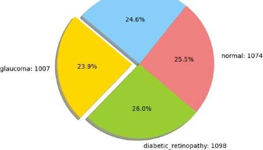
Fig.1. Class distribution in dataset

• A.    Data Prepossessing Batch Normalization

  Batch normalization [16] i s performed following the EfficientNetB3 feature extractor to normalize the 1536dimensional feature vector. It normalizes the features and consequently adjusts their mean and variance for each batch, minimizing internal covariate shift. That serves to stabilize and accelerate training, enables the use of larger learning rates, and in- creases the flow of gradients. Batch normalization also introduces two learnable parameters: scale and shift, which allow the model to learn the optimal feature distributions. In general, it improves the stability of the training and perform regularization effect in addition to dropout.

• B.    Transfer Learning

The model applies transfer learning [17] b y using EfficientNetB3, which has been pre-trained over the ImageNet dataset, as a feature extractor. Rather than starting from scratch, it uses pre-trained weights which have already learned general image patterns. The base EfficientNetB3 extracts meaningful features from the retinal images, and only the classification layers affixed are trained on the respective dataset. This method not only accelerates training, but also allows greater accuracy, especially with limited data.

• C.    Regularization

To prevent overfitting, we also apply regularization techniques [18], u sing weight decay L2 and regularization L1 over the biases. The L2 version of the regularizer will discourage very large weights, and the L1 version of the regularizer will help with the selection of features (promoting sparsity). These techniques help to handle model complexity, which allows models to generalize better to unseen data.

• D.    Dropout

• 3.2.    Proposed Machine Learning Model

  The image classifier model is derived from the EfficientNetB3 architecture, a cutting-edge efficient CNN that scales network breadth, depth, and resolution in an efficient manner. RGB images of size 224×224 pixels are fed into the model as input, in adhering to EfficientNetB3 input expectations. The model basis lies in EfficientNetB3 that has been pretrained over the ImageNet dataset with removal of classification heads (include-top=False). The base framework of this model transforms input images through a series of convolution layers and Mobile Inverted Bottleneck Convolution (MBConv) blocks to extract complex hierarchical feature representations at diversified scales. Subsequently, a global max pooling layer squeezes spatial feature maps to a settled size of 1536-dimensional feature vector, encapsulating predominant information of input image. In an effort to add stability to training and to boost overall performance of model, it has a Batch Normalization layer in place succeeding to that of EfficientNetB3 basis. After this layer, a densely connected layer of 256 neurons has been included with L1 and L2 regularization in place to avoid overfitting as well as model generalization. The layer has an activation function for ReLU which renders the model non-linear. There has been utilization of Dropout layer with rate 0.45 for regularization through dropout of neurons randomly during their training and hence their inter- dependencies. The output layer has a Dense layer with neurons equal to target classes (four in this case), with softmax activation function for classifying to create a class of probability distribution. There has been usage of Adamax optimizer with an initialization of learning rate of 0.001 for multi-class classification problem through categorical crossentropy loss, and monitored through accuracy metrics while it trains.

• 3.3.    Model Selection Rationale

The model also comprises a 0.45 rate dropout layer after a 256 dense layer. Dropout [19] h appens during training time by deactivating randomly 45% of the neurons in this layer. By making it more difficult for neurons to learn from one another, this prevents the model from overfitting. Through this, the model learns more general and stable features. Dropout is disabled during inference such that all the neurons work together to make the final prediction.

Table 1. Architecture of EfficientNetB3 model

Layer Type	Output Shape	Parameters / Details	Notes
Input	(224, 224, 3)	—	Input image size and channels
EfficientNetB3 (base)	(None, 1536)	Pretrained on ImageNet	Main feature extractor, convolutional backbone with global max pooling
BatchNormalization	(None, 1536)	˜6,144 (depends on shape)	Normalizes output for stability

Dense	(None, 256)	"393,472 (weights + bias)	Fully connected layer with L1 & L2 regularization and ReLU activation
Dropout (0.45)	(None, 256)	0	Regularization to reduce overfitting
Dense (Softmax)	(None, 4)	"1,028	Output layer for 4-class classification

The deep learning architectures evaluated in this study were selected to represent diverse design strategies and performance characteristics in image classification. EfficientNetB3 was chosen for its compound scaling approach that balances accuracy and efficiency. ResNet50 and DenseNet121 were included due to their proven ability to learn deep and discriminative features in medical imaging tasks. MobileNetV2 was selected to assess performance under computational constraints, making it suitable for deployment in resource-limited settings. VGG16, although an older architecture, was included as a classical baseline to provide a comparative reference against more recent models. The previously included Recurrent Neural Network (RNN) was removed, as RNNs are not well-suited for static image classification tasks. This selection enables a comprehensive comparison of accuracy, efficiency, and architectural complexity across different CNN designs.

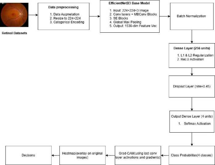
Fig.2. Model diagram of the proposed EfficientNetB3 architecture employed in this study for eye disease detection and classification

Fig. 2. delineates overall design as well as explainability pipeline of our classification system for retinal images. For the retinal datasets, images have to undergo data preparation with procedures for data augmentation to expand training data, make all the photos the same size, 224×224 pixels, which is the right size for the model, and categorical encoding of class labels. The preprocessed images are fed into the base model of EfficientNetB3, which consists of a convolutional neural network architecture of convolutional layers and MBConv or Mobile Inverted Bottleneck Convolution and Squeeze- and-Excitation (SE) blocks. The model extracts a 1536-dimensional feature vector via global max pooling. The feature vector undergoes Batch Normalization to normalize it and stabilize and speed up training through normalization of layer inputs. Normalized features are fed into a Dense layer of 256 units with L1 and L2 regularization to avoid overfitting and ReLU activation for the introduction of non-linearity. There is also a Dropout layer of 0.45 to avoid overfitting through dropout of neurons at random during training. There’s a final Dense layer of four units that employ a softmax activation function to give class probabilities for the four retinal diseases. Grad-CAM for interpretability enhancement analyzes the predictions of the model and computes gradients with respect to activations of the terminal convolutional layer to generate heatmaps. The heatmaps are overlaid over source images in an endeavor to highlight through visual means key areas that are most important in terms of making the categorization decisions.

4.    Implementation and Experimental Setup 4.1.    Metrics for Model Evaluation

We utilize the following measures to see how well our proposed model works:

• A.    Confusion Matrix

The confusion matrix [20] i s a chart that shows how many times each category shows up in a dataset. These come in four types: True Positive (TP), False Negative (FN), False Positive (FP), and True Negative (TN).

Table 2. Confusion matrix displaying the performance of the EfficientNetB3 model

Actual Class	Predicted Class
	Positive (1)	Negative (0)
Positive	True Positive (TP)	Negative (FN)
Negative	Positive (FP)	True Negative (TN)

• B.    Accuracy

The accuracy is the number of accurately predicted cases (true positives and true negatives) divided by the total number of examples looked at. It indicates you how accurate a categorization model is in general. The way to figure it out is:

Accuracy =

TP+TN

TP+TN+FP+FN

x 100%

C. Precision

Precision [21] t ells us what percentage of the images the model correctly identified as positive out of all the images it considered were positive. You may figure out precision by:

Precision =----x 100%

TP+FP

• D.    Recall

The recall [22] i s the quantity of samples that were correctly classified positive divided by the total amount of properly categorized positive specimens and incorrectly classified negative samples. It checks to see how well a model can find all the good examples. The model is more sensitive and has fewer false negatives if it has a higher recall. The formula for figuring out recall is:

_           TP

Recall = ^^x x 100%

• E.    F1 Score

The F1 score [23] i s only one number that finds the harmonic mean of accuracy and recall. It seeks a balance between precision and recall, which tells you how precise a model is, particularly when the classes are not the same size. You can find out the F1 score by:

F1— score =

2 x

Precision+Recall

x 100%

• F.    Kappa Score

The kappa score [24], o ften called Cohen’s kappa, shows how much two raters or classification techniques agree with one other, taking into account the likelihood that they may agree by chance. It can be anywhere from -1 to 1, with 1 being complete agreement, 0 meaning no better than random chance, and negative values meaning disagreement. Kappa score can be considered as:

Kappa = ^P^                            (5)

1-P e

• G.    ROC Curve

The ROC curve [25] s hows the rate of true positives and false positives for differing levels of threshold to assess the effectiveness of a binary classifier. The AUC (Area under Curve) of this plot gives a single measure that shows how effective in class separation a model is. Larger AUC shows higher discrimination.

• H.    Logarithmic Loss

• 4.3.    Interpreting the Model Performance

• 4.4.    Experimental Setup

Logarithmic loss, or log loss, measures how well a classification model’s predicted probabilities match the actual labels. It penalizes false predictions more when the model is confident but wrong, producing a lower loss for accurate and confident predictions. Lower log loss values indicate better performance of the mode l [26] . Log loss can be calculated as:

LogLoss = -^Т^.Т^Хц x log (p^)                         (6)

Explainable AI The goal of using Explainable AI [27] t o make machine learning algorithms more clear and understandable for human users, fostering trust in AI systems by clarifying their managerial processes. This is of particular significance in sectors such as autonomous transportation and healthcare. where AI decisions can matter a great deal. XAI enables users to make sense of how an AI model functions, establishes transparency in explaining its predictions, in- creases its trustworthiness, and uncovers biases to enable fair decision-making. A crucial methodology employed in XAI is Grad-CAM that enhances CNNs’ interpretability. Grad-CAM makes a visual explanation by showing which aspects of the image are crucial for the model’s choice. It is to find the gradients of the target class score in relation to the feature maps, and then average over the plane of the feature maps to obtain the weight of them. The end product is a heat map which gives a visual indication of the important regions of the image. Furthermore, in medical AI, for example, in predicting eye diseases, the use of Grad-CAM was very useful. It assists the clinicians in knowing which parts of an eye scan image are affect the diagnostic decisions of the model keeping medically meaningful features first. This interpretability increases confidence in AI diagnosis, and validates the efficacy of the model, which helps ensuring proper patient care.

To demonstrate our proposed model, we have to apply some setups which are given below:

• A.    Platform

The experiments were conducted in a Python 3.10 environment using Keras 2.4 and TensorFlow GPU 1.8. The hardware included a Intel Core i7 v8 computer running Windows 11 @3.10GHz CPU, 12GB RAM, and an NVIDIA Geforce GPU.

• B.    Training and Validation

We trained an EfficientNetB3 model to categorize patches utilizing various hyperparameters. The model underwent training for 20 epochs, with a sample size of 10 and a learning rate of 0.001. Training was ended if no progress was observed after three reductions in the learning rate. If the validation loss did not decrease for one epoch, the learning rate was halved. The data was divided into three categories: training (80%), validation (10%), and testing (10%). No cross-validation was conducted, and the Adamax optimizer was utilized with its default parameters.

• C.    Dataset Separation

5.    Result Analysis and Discussion 5.1.    Performance Evaluation of Models

The dataset was divided into training, validation, and test sets in an 80-10-10 ratio after file locations and associated labels were defined. We developed data generators for training, validation, and testing. TensorFlow classes took care of data augmentation and preprocessing. The training data was mixed up, but the test data was not.

Based on performance metrics, results are analyzed below:

• A.    Accuracy

Table 3. shows that EfficientNetB3 achieved the highest accuracy at 97.00%, followed by MobileNet-V2 at 95.00%, and DenseNet121 at 94.00%. ResNet50 has accuracy of 91.00%, while VGG16 had the lowest accuracy at 87.06%.

Table 3. Comparison of classification accuracy across different deep learning models. EfficientNetB3 exhibit the highest performance

Model Name	Accuracy (%)
EfficientNetB3	97.00
ResNet50	91 . 00
VGG16	87 . 06
MobileNet-V2	95 . 00
DenseNet121	94 . 00

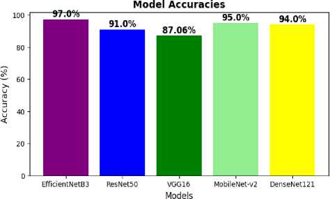
Fig.3. Comparison of classification accuracies across different models, with EfficientNetB3 achieving the highest accuracy

• B.    Precision

Table 4. d isplays precision scores for different eye conditions. DenseNet121 and EfficientNetB3 excelled in precision for Cataract (97% and 96%, respectively). For Diabetic Retinopathy, EfficientNetB3, ResNet50, and DenseNet121 all achieved perfect scores. DenseNet121 led for Glaucoma (97%), and EfficientNetB3 had the highest precision for Normal conditions (94%).

Table 4. Performance comparison of models based on precision scores for cataract, diabetic retinopathy, glaucoma, and normal classes

Model	Cataract	Diabetic Retinopathy	Glaucoma	Normal
EfficientNetB3	0 . 96	1 . 00	0 . 97	0 . 94
ResNet50	0 . 97	0 . 99	0 . 85	0 . 89
VGG16	0 . 89	0 . 95	0 . 86	0 . 86
MobileNet-V2	0 . 86	0 . 88	0 . 85	0 . 85
DenseNet121	0 . 93	0 . 94	0 . 93	0 . 87

C. Recall

Table 5. shows recall scores where EfficientNetB3 led across all classes with scores of 0.99 for Cataract, 1.00 for Diabetic Retinopathy, 0.93 for Glaucoma, and 0.95 for Normal. DenseNet121 and ResNet50 also performed well, with high recall across various conditions. VGG16 had a lower recall for Glaucoma.

Table 5. Recall scores by model and class

Model	Cataract	Diabetic Retinopathy	Glaucoma	Normal
EfficientNetB3	0 . 99	1 . 00	0 . 93	0 . 95
ResNet50	0 . 94	0 . 99	0 . 88	0 . 88
VGG16	0 . 95	1 . 00	0 . 75	0 . 89

MobileNet-V2	0 . 92	0 . 88	0 . 89	0 . 90
DenseNet121	0 . 88	0 . 93	0 . 85	0 . 94

D. F1 Score

Table 6. indicates F1 scores where EfficientNetB3 consistently performed best, especially in Cataract (0.98) and Diabetic Retinopathy (1.00). DenseNet121 showed strong results for Normal (0.91). VGG16 and MobileNetV2 showed varied results across classes.

Table 6. F1 Scores by model and class

Model	Cataract	Diabetic Retinopathy	Glaucoma	Normal
EfficientNetB3	0 . 98	1 . 00	0 . 95	0 . 95
ResNet50	0 . 95	0 . 99	0 . 86	0 . 88
VGG16	0 . 92	0 . 97	0 . 79	0 . 87
MobileNet-V2	0 . 94	0 . 93	0 . 88	0 . 88
DenseNet121	0 . 93	0 . 85	0 . 88	0 . 91

• 5.2.    Analysis of Test and Validation Curve

For this experiment, the base model efficientNetB3 is augmented with extra layers of Batch Normalization layer, Dense layer of 256 units to regularize well, and a Dropout layer of rate 0.45. The Dense layers use ReLU activation function for bringing in non-linearity. There are data splits: 80% for training, 10% for validation, and 10% for testing. Adamax optimizer with a learning rate initialized at 0.001 trains the model. If the accuracy does not improve after some epochs (patience), a callback function monitors the training and reduces the learning rate by a factor of 0.5. The training batch size is 32, and the training runs for a maximum of 20 epochs. Also, pretrained EfficientNetB3 layers are also finetuned so that the model can work even better on the target dataset. The left plot shows that both the training loss and the validation losses are declining regularly. That means that the model is learning how to reduce the number of errors it commits when it makes predictions. The minimum validation loss occurs at epoch 19, which is when the model generalizes optimally to new observations. Right training accuracy just continues to improve, rising above 99% in the final epochs. Validation accuracy peaks at about epoch 15, when it is about 95%. This indicates that the model is fitting optimally on the validation set before beginning too just slightly overfit. Loss indicates how much model’s predicted probabilities are deviated from actual labels, while accuracy indicates the proportion of correct predictions. These were calculated after each epoch for training and validation sets.

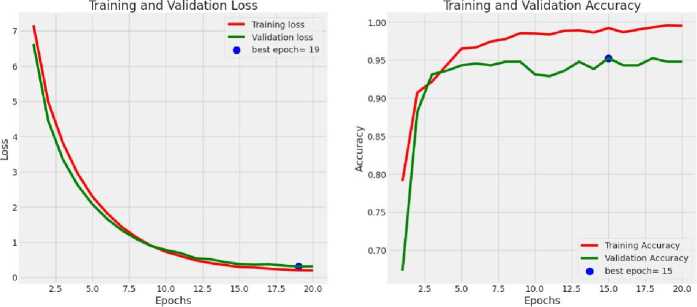
Fig.4. Test and validation curves depicting the model’s performance over training epochs, showing the accuracy and loss trends for both the training and validation datasets

• A.    ROC and AUC Analysis

Fig.5. shows the AUC scores and ROC contours for the multi-class classification of eye diseases. EfficientNetB3 demonstrated exceptional performance with an AUC score of 1.00 for all classes: cataract, diabetic retinopathy, glaucoma, and normal. This indicates excellent discrimination between classes.

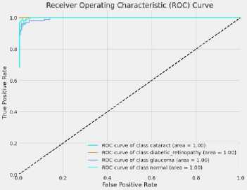
Fig.5. ROC curve and AUC of the EfficientNetB3 model, demonstrating its excellent classification performance with an AUC value of 1.00

• B.    Logarithmic Loss

Table 7. present the log loss for each model. EfficientNetB3 achieved the lowest log loss of 0.10, indicating the most accurate prediction performance and fewer errors. ResNet50 followed with a log loss of 0.21. VGG16, MobileNetV2, and DenseNet121 had higher log losses of 0.26, 0.59, and 0.56, respectively, with MobileNetV2 and DenseNet121 being less reliable compared to the top models.

Table 7. Logarithmic loss of different models

Model Name	Logarithmic Loss EfficientNetB3
ResNet50	0 . 10
VGG16	0 . 21
DenseNet121	0 . 56

• C.    Kappa Score Analysis

Table 8. s hows Cohen’s Kappa scores, the maximum Kappa Score of 0.95 was attained, indicating the most favorable agreement between the predicted and actual classifications by EfficientNetB3. ResNet50 had a Kappa Score of 0.88, demonstrating good predictive ability but slightly lower than EfficientNetB3. VGG16 scored 0.86, while MobileNetV2 and DenseNet121 had the lowest Kappa Scores of 0.61, indicating poorer performance.

Table 8. Kappa scores of different models

Model Name	Kappa Score
EfficientNetB3	0 . 95
ResNet50	0 . 88
VGG16	0 . 86
MobileNet-V2	0 . 61
DenseNet121	0 . 61

• D.    Confusion Matrix Analysis

Fig.6. The model was evaluated on a test set comprising 422 retinal images randomly selected from the dataset. As depicted in Figure 5, the confusion matrix shows high values along the diagonal for all four classes: cataract, diabetic retinopathy, glaucoma, and normal; indicating strong classification accuracy across categories. The results demonstrate that the EfficientNetB3-based model effectively distinguishes between different retinal disease types, confirming its robustness and reliability on unseen data. Here’s a breakdown:

• •    Cataract: 103 correct predictions, 1 misclassified as normal.

• •    Diabetic Retinopathy: Perfect accuracy with 110 correct predictions and no misclassifications.

• •    Glaucoma: 94 correct predictions, with 2 instances misclassified as cataract and 5 as normal.

• •    Normal: 102 correct predictions, with 2 instances misclassified as cataract and 3 as glaucoma.

  

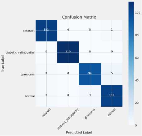
Fig.6. Confusion matrix

The darker shades on the matrix indicate a higher number of correct predictions, while lighter shades represent mis-classifications. EfficientNetB3 performs exceptionally well, especially for diabetic retinopathy, but there is some room for improvement in distinguishing glaucoma from cataract and normal classes.

• E.    Grad-CAM Visualization

• F ig.7. d epicts a Grad-CAM heat map superimposed on a retinal fundus photograph. The heat map helps in visualizing which areas the image’s components are the most significant in the model’s predictions:

• •    Optic Disc: The bright yellow-white area represents the optic disc, a key landmark where the optic nerve exits the eye.

• •    Retinal Blood Vessels: The red and purple lines radiating from the optic disc are blood vessels supplying the retina.

• •    Central Macula: The hyperpigmented central macula, appearing more red and yellow, may indicate increased metabolic activity or a pathological process.

The Grad-CAM method was used to interpret the model’s predictions. For Glaucoma, the heatmaps highlighted the optic disc, which is a key feature in identifying glaucoma. For Diabetic Retinopathy, the model focused on areas with microaneurysms, which are characteristic signs of the disease. The Grad-CAM visualizations did not highlight irrelevant areas such as the background or eyelashes, ensuring that the model’s attention was directed towards clinically significant regions.

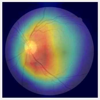
Fig.7. Grad-CAM visualization showing the regions of interest in the eye images that contributed most to the EfficientNetB3 model’s predictions

F. Visualization

The full visualization process was done by using flask on backend. Total Visualization system was implemented using VSCode IDE. A website is locally run by an IP address where an interface is responsible for the classification of eye diseases. after hitting IP address, a website is opened. there is a space where users can upload images to classify. after providing the image the website shows the output result of the image. All those happen based on the EfficientNetB3 model which helps to classify images.

INFO:werkzeug:WARNING: This is a development server.

* Running on http://127.В.6.1:5800

INFO:werkzeug:Press CTRL+C to quit

INFO:werkzeug: * Restarting with stat

Fig.8. Local website’s IP address

Eye Disease Classifier

| Choose File | No File chosen

Upload and Predict

Fig.9. Web page design showcasing the user interface for the eye disease detection system

Prediction Result

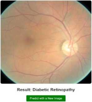
Fig.10. Prediction results of the EfficientNetB3 model, showcasing the model’s classification outcomes for different eye diseases based on the input medical images

• 5.3. Discussion

6. Conclusions and Future Works

EfficientNetB3-based model outperformed other DL model in classifying retinal disease because it has a compound scaling approach that achieves an optimal compromise among network depth, width, and input resolution. We downsam-pled images to 224×224 to maintain input size same as that of pretrained input. We also used ImageNet weights to reduce convergence time and get better feature learning. The model performed well and was stable with learning rate of 0.001, Adamax optimizer, batch size of 10 with training running for 20 epochs. Regularization (L1=0.006, L2=0.016), dropout (0.45), and batch normalization all worked well to reduce overfitting and make training for it more robust. The model performed well, yet it remains sensitive to noise and variation of picture. Grad-CAM interpretability of it yet has to be proven to make sure that it has clinical utility. In times to come, various big-data clinical databases from other hospitals will be utilized to challenge the model to function under varying demographics, modalities of imaging, and settings. It is also important to see how well performs with poor or anomalous pictures of eyes. Also, engaging ophthalmologists and other doctors in user testing will allow us to ascertain how informative and descriptive Grad-CAM-based explanations are. Individual input can make it simpler for model to understand over time in making it simpler to use in clinic.

Our work focused on employing explainable AI and machine learning in diagnosing eye disorders. The highest-performing model was the EfficientNetB3 model. With an overall accuracy of 97.003%, EfficientNetB3 significantly outperformed other models in precisely classifying four separate eye disorders. In each class, the model reliably possessed excellent F1 scores, precision, and recall. F1 values, for example, ranged from 0.95 to 1.00, precision levels ranged from 0.94 to 1.00, and recall levels ranged from 0.93 to 1.00 (Tables 4, 5, and 6). The model is better at accurately identifying and discriminating between cataract, diabetic retinopathy, glaucoma, and normal situations than ResNet50, VGG16, MobileNetV2, and DenseNet121. We better comprehended the decision-making process of the model through the application of explainable AI methods such as Grad-CAM, an indispensable tool in medicine. Knowing how a model came to its conclusion is just as important in clinical practice as knowing what that conclusion is. On the whole, results show that ophthalmic patients can make better and more confident choices through employing the best of machine learning models with explainable AI that do not only give extremely correct diagnosis but in addition make it understandable how predictions are arrived at.

Furthermore, the proposed system shows strong potential for real-world deployment in large-scale screening programs and telemedicine applications, particularly in remote and resource-limited regions where access to ophthalmologists is re- stricted. By providing automated disease classification along with visual explanations, the system can function as an effective clinical decision-support tool, assisting ophthalmologists in early diagnosis, prioritization, and remote patient monitoring. Overall, this approach contributes toward improving accessibility, efficiency, and reliability in ophthalmic healthcare delivery.

In the future, we will work on combining 3D retinal analysis with OCT data, making the software more accessible throughout the world by adding support for several languages and localised interfaces, and balancing datasets with synthetic data created by GANs. Time-series analysis can be used to keep track of how a disease is getting worse so that treatment can start early. A cloud-based, scalable deployment architecture will cut down on hardware expenses, while integrating EHRs will add patient data to the system. Finally, making sure that bias and fairness are present in all groups will be very important.

All the Declarations and StatementsAuthor Contributions Statement

Sadikur Rahman Sadik – Data Curation, handled data acquisition, dataset preprocessing, and implemented the research model. Model Training, Validation, and Performance Evaluation: Led the model training process, validated results using standard metrics, and benchmarked performance against existing methods.

Md. Abdul Halim Khan – Visualization, Conceptualization, Methodology, Writing – Drafted the initial manuscript, contributed to the literature survey, and documented the technical background of the study.

Samsuddin Ahmed – Supervision: Proposed research ideas, constructed the overall framework, and supervised project execution. Writing – Review and Editing, and Project Management: Reviewed and edited the manuscript, ensuring clarity and coherence and helped coordinate project milestones and deadlines.

Atiqur Rahman – Formal Analysis, Visualization, and Statistical Analysis: Performed in-depth analysis of experimental results, prepared performance charts, ensured the statistical robustness of the evaluation and helped coordinate project milestones and deadlines.

Sadia Enam – Formal Analysis, Visualization, and Statistical Analysis: Performed in-depth analysis of experimental results, prepared performance charts, ensured the statistical robustness of the evaluation and helped coordinate project milestones and deadlines.

Md. Toukir Ahmed – Supervision: Proposed research ideas, constructed the overall framework, and supervised project execution. Writing – Review and Editing, and Project Management: Reviewed and edited the manuscript, ensuring clarity and coherence, and helped coordinate project milestones and deadlines.

All authors have read and agreed to the published version of the manuscript.

Conflict of Interest Statement

The authors declare no conflicts of interest.

Funding Declaration

We received no external funding for this research.

Data Availability Statement

All data utilized in this study were obtained from publicly available sources. No new datasets were generated or analyzed.

Ethical Declarations

The authors should declare the following: Statements of ethical approval for studies involving human subjects and/or animals.

Acknowledgments

Declaration of Generative AI in Scholarly Writing

During the preparation of this work, the authors used different AI tools to improve the language and readability. After using these tools/services, the authors reviewed and edited the content as needed and took full responsibility for the content of the publication.

Abbreviations

The following abbreviations are used in this manuscript:

ML – Machine Learning

AI – Artificial Intelligence

XAI – Explainable Artificial Intelligence

CNN – Convolutional Neural Network

Grad-CAM – Gradient-weighted Class Activation Mapping

TP – True Positive

FP – False Positive

TN – True Negative

FN – False Negative

ROC – Receiver Operating Characteristic

AUC – Area Under Curve

CAD – Computer -Aided Design

SHAP – Shapely Additive explanations

LIME – Local Interpretable Model-agnostic Explanations

MBConv – Mobile Inverted Bottleneck Convolution

DL – Deep Learning

ReLU – Rectified Linear Unit