Hoff's model on a geometric graph. Simulations

Take a finite connected oriented graph G = G(V; E) with vertex set V = {V,} and edge set E = {Ej} . Associate to the each edge Ej two positive integers lj. dj E R₊. which have physical meaning in the context of our problem: the length and area of the cross-section of the edge.

Consider Hoff’s model of the dynamics of H-beam constructions. On each edge Ej we set up the generalized Hoff ecpiation

AjUjt + Ujxxt = a i jUj + a 2 juj + ... + anju^{2n 1} , n E N ,               (1)

and at each vertex we impose the boundary conditions uj (0,t) = Uk(0,t) = Um(lm, t) = Up(lp ,t),   Ej ,Ek E Ea(V,),Em,Ep E Eш(V,),   (2)

j :

E

djUj_x (0 , t )

d_mU_mx ( l_m , t ) = 0 ,

Ej eE^a ( Vi )

m :

EE' ( Vi )

where Ea (V,) aiid Eш (V,) are the sets of edges with the source and target vertex V, respectively. The parameters Aj E R+ correspond to the load on beam j, and the parameters asj E R fc>r s = 1,2, ...,n characterize the material of beam j. The unknown functions Uj (x,t) о f x E (0, lj) aiid t E R specify the defl ection of beam j from the vertical direction.

The direct problem consists in finding the vector function u = ( u 1 , u2, ...,Uj,... ), each component uj ( x,t ) of which satisfies the continuity condition (2) and the flow balance condition (3). Besides, the components uj ( x, t ) must satisfy the Cauchy initial conditions

Uj ( x, 0) = Uj ₀( x ) ,   x E (0 , lj ) .

or the Showalter-Sidorov initial conditions

∂ ²

I Xj + — ( Uj ( x, 0) - Uj o( x )) = 0 , x E (0 ,lj).

The inverse problem (in the case n = 2) consists in finding the solutions Uj to (1) and the unknown coefficients aj = a 1 j a nd ej = a 2 j using the additional measurements

aj U oj (0) + ej U 0 j (0) = фj,   aj U oj ( lj ) + ej U 0 j ( lj ) = ^j, where фj and rj reflect the change of the rate in buckling dynamics at the endpoints of the beam at the initial moment.

The paper aims to generalize the results of [1,2] to the case of the inverse problem for Hoff’s model with the Showalter-Sidorov conditions and to develop numerical algorithms for solving the stated problems. Hoff’s ecpiation belongs to the class of semilinear Sobolev-type equations; for this reason we use here the theory of degenerate semigroups and relatively p -bounded operators. For more details concerning the theory of semigroups and Sobolev-type ecpiations, as well as Cauchy and Showalter-Sidorov problems, see [3-7].

1.    Hoff’s Model

Following [1,2], reduce (l)-(4) to the Cauchy problem u (0) = u ₀, and (l)-(3), (5) to the Showalter-Sidorov problem L ( u (0) — u ₀) = 0 for the semilinear Sobolev-type equation LU = Mu + N ( и ). Consider the Hilbert space L2(G) as well as two spaces U and F with the natural structure of a Banach rather than Hilbert space. Define the operators L, M, N : U ^ F as

(Lu,v) = ^^ dj / ( XjUjVj — UjxVjx ) dx, (Mu,v) = ^^ a 1 jdj I Ujvjdx, j ⁰                                                        j             ⁰

(N(и) ,v) = ^2 dj ^a2j j ujVjdx + ... + anj j uj2n-1vjdx , where (•, •) is the inner product on L2(G). For’ all a2j,a3j,...,anj E R we 1 rave N E G”(U; F). The operators L and M lie in L(U; F), that is, are linear and continuous. Moreover. L is Fredlrolin (that is. ind L = 0). wFile M is comp act and (L, 0)-bounded whenever ker L = {0} оr ker L = {0} and all coefficients a 1 j are nonzero and of the same sign.

Let us state the main results as theorems on the solvability of direct and inverse problems in the case of the Cauchy problem and Showalter-Sidorov problem for Hoff’s equations on the graph (the first three theorems are proved in [1,2]).

• Theorem 1.

• (i)    If ker L = { 0 } then tin?, phase space, of (1) is Я.

• (ii)    If ker L = { 0 }, all a 1 j are nonzero and of the same sign as all nonzero coefficients asj for s = 2 , ...,n then the phase space of (1) is the simple manifold

M = {u E Я : (Mu + N(u), xk) = 0, missing} where, ker L = span{xk : k = 1,2,■ ■■, l} is an L2(G)-orthonormal basis о/ker L identified with a basis of cokerL.

Denote by D the set of admissible values of the vectors ф and fi for which the solutions to the inverse problem are the coefficients aj a nd ej of the same sign ( aj >  0, ej >  0 or aj <  0. ej <  0 for all j ). The struct!rre of the set D is described in [2].

• Theorem 2.

• (i) If ker L = { 0 } then ,for all u 0 E Я anul фj. fij E R satisfging u 0 j (0) = 0. u 0 j ( lj ) = 0. u 0 j (0) = ±u 0 j ( lj ) фj u 0 j ( lj ) = fiju 3 j (0), a nd фj u 0 j ( lj ) = fiju 0 j (0) there exists a unique solution to the inverse problem (l)-(f), (6).

• (h) If ker L = { 0 } then , for all ф/ф E D an ul u 0 = ( u ₀₁ , u ₀₂ , ...,u 0 j,... ) E Я sat isfging u о j (0) = 0. u о j ( lj ) = 0. u о j (0) = ±u о j ( lj ). and.

  lj i = d I

  
  

  (⁽ фj^u 0 j ^{( l}j ) - ^fij^u 0 j ^{(0)) u} 0 j + ^{( fi}j^u 0 j ⁽⁰⁾ - фj^u 0 j ^{( l}j )) ^u 0 j) ^dx,Xk

  
  
  
  

  = 0 ,

  
  

there exists a unique solution u E Я, aj, ej E R \{ 0 } to the inverse problem fl)-(4), (6) with ajej E R₊.

• Theorem 3.

• (i)    If ker L = { 0 } then for all u ₀ E Я there exists a unique solution to the Showalter-Sidorov problem (l)-(3), (5).

• (ii)    If ker L = { 0 } and all co efficients asj = 0 for s = 1 , ...,n are of the same sign, then for all u 0 E Я there exists a unique solution to the Showalter-Sidorov problem (l)-(3), (5).

• Theorem 4.

• (i)    If ker L = {0} then ,for all u₀E Я. фj. fij E R satisfging u₀j(0) = 0. u₀j(lj) = 0. u 0 j (0) = ±u 0j (lj), фj u 0 j (lj) = fiju 0 j (0), a nd фj u₀j (lj) = fiju₀j (0) there exists a unique solution to the inverse problem (l)-(3), (5), (6).

• (ii)    If ker L = {0} then for ₀E Я satis.fging u₀j(0) = 0. u0j(lj) = 0. a/nd u0j(0) = ±u₀j(lj) there, exists a icniquc. solution u E Я. aj. ej E R\{0} to the inverse problem (l)-(3), (5), (6) with ajej E R₊.

2.    The Results of Simulations

Proof, (ii) Suppose that u ₀ E Я and the conditions u ₀ j (0) = 0, u ₀ j ( lj ) = 0, u ₀ j (0) = ±u 0 j ( lj ) are fulfilled. Then there exists a unique pair of coefficients aj ar id ej satisfying (6). The condition ф,fi E D ensures that ajej >  0 for all j. Moreover, by the construction of D. all coefficients aj are nonzero and of the same sign as the nonzero coefficients ej'- Hence, the hypotheses of claim (ii) of Theorem 3 hold, and so there exists a unique solution u E Я. aj. ej E R \{ 0 } to the inverse probleni (l)-(3). (5). (6) with ajej E R₊.

________________________________________________________________□ 86 Вестник ЮУрГУ. Серия « Математическое моделирование и программирование м

Basing on the theoretical results for Hoff’s model on a graph, we wrote a software bundle in the symbolic algebra package Maple 15.0. It enables us to:

• (1)    find numerical solutions to direct and inverse problems with given coefficients Xj, aij, фj, a nd ^j as Galerkin sums of the first few eigenfunctions;

• (2)    draw the graphs of the solutions to Hoff’s model on a graph;

• (3)    draw the phase space of Hoff’s model on a graph.

Example 1. Take the graph G with three vertices V 1, V 2, a nd V3 and two adjacent edges E 1- of Itength 1 1 = n and area, d i = 1 of the. cross-section, and E ₂. of It-ngth 1 ₂ = n and area, d₂ = 1 of the. cross-section.

Consider on G the equations of Hoff's model with X 1 = 1. X ₂ = 1. a 11 = — 10. a 2i = — 0 , 5. a 12 = — 0 , 5. a 22 = — 0 , 19:

{ u 1 1 + u 1 xxt + ¹⁰ u 1 + ⁰ , ⁵ u 1 = ⁰

[ u 2 1 + u 2 xxt + 0 , 5 u 2 + 0 , 19 u 2 = 0 .

The continuity conditions are u 1( n, t ) = u ₂(0 , t ), and the flow balance conditions are u . x (0 , t ) = 0, u 1 _x ( n,t ) = u _{2 x} (0 , t ), a nd u _{2 x} ( n, t ) = 0. Seek the solution to (7) as the Galerkin sums

NN uГ ^{( x,t} ) = ^ vi ⁽ t ) ⁽ x ) , uN ^{( x,}t ) = ^ vi ⁽ t ) Ci ⁽ x ) , i =1                                 i =1

where xi ( x ) = ( Ci ( x ) , Zi ( x )) ^are the eigenfunctions of the Sturm-Liouville problem on the graph. For N = 3, the eigenvalues and eigenfunctions are

P 1 = 1 , X 1 = ⁽¹ , 1) ,

T2 = 0, 75, x2 = (cos(2), — sin(2)), p3 = 0, x3 = (cos x, — cos x), so we look for the solution in the form u 1(x, t) = v 1(t) + v2(t) cos x + vз(t) cos(2), u2 (x, t) = v 1 (t) — v2 (t) cos x — v3 (t) sin(2).

In the case X 1 = X ₂ = 1 claim (ii) of Theorem 1 applies because 0 G a ( L ).

Multiplying (7) by the functions xk f°^r k = 1 , 2 , 3, we obtain the system of differential

Table 1

The numerical solution to (8) with initial data v 1(0) = - 0 , 01 ,v 2(0) = - 0 , 01 ,v 3(0) = 0 , 02

t v 1( t) v 2( t ) v 3( t) 0 —0, 01 -0,00738 0,02 0,05 —0,010116 —0,006685 0,018122 0,10 —0,009997 —0,006173 0,016736 0,15 —0,009748 —0,005774 0,015652 0,20 —0,00943 —0,005443 0,014757 0,25 —0,00908 —0,005159 0,013985 0,30 —0,008718 —0,004905 0,013296 equations

0 , 4786 v 2( t ) v з( t ) + 0 , 248 v 3( t ) + 6 , 2 v з( t ) + 0 , 62 v2(t ) v з( t ) +

+ 1 , 736 v i( t ) v ₂( t ) v з( t ) + 1 , 626 v ₂( t ) v 3( t ) + 16 , 808 v ₂( t )+

+3 , 252 v 2( t ) v2(t ) + 0 , 813 v 3( t ) + 1 , 626 v i( t ) v 2( t ) = 0 ,

• 1 , 24 v i( t ) v ₂( t ) v 3( t ) + 18 , 6 v 3( t ) + 0 , 413 v 3( t ) + 0 , 868 v 2( t ) v 3( t )+

< +1 , 86 v 2( t ) v 3( t ) + 33 , 615 v i( t ) + 3 , 252 v i( t ) v 2( t ) + 6 , 283 v i( t ) +                      (8)

+2 , 168 v 3( t ) + 1 , 626 v ₂( t ) v 2( t ) + 3 , 252 v ₁( t ) v 2( t ) = 0 ,

• 0 , 868 v i( t ) v ₂²( t ) + 18 , 6 v i( t ) + 1 , 24 v i ( t ) v ₃² ( t ) + 0 , 744 v 2( t ) v ₃²( t ) + 0 , 62 v _i² ( t ) v 2 ( t )

+0 , 159 v 3( t ) + 6 , 2 v ₂( t ) + 0 , 62 v 3( t ) + 1 , 626 v 2( t ) v ₃( t ) + 3 , 252 v 2( t ) v ₃( t )

+16 , 808 v ₃( t ) + 3 , 252 v ₁( t ) v ₂( t ) v ₃( t ) + 0 , 813 v 3( t ) + 2 , 356 v ₃( t ) = 0 .

Figure l.a depicts its phase space.

Let us solve the Showalter-Sidorov problem for (8) with the data v 1(0) = — 0, 01, v 2(0) = — 0, 01, a nd v3(0) = 0, 02, which corresponds to the initial condition u 1(x, 0) = — 0, 01 — 0, 01 cos x + 0, 02 cos(2)

u ₂( x, 0) = — 0 , 01 — 0 , 01 cos x — 0 , 02 sin(^)

for (7). Table 1 lists some values of the solution to (8) in a neighbourhood of the point t = 0, while Figure l.b depicts its graph.

Consider on G the equations of Hoff's model with a 11 = — 1. a ₂₁ = — 0 , 5. a ₁₂ = — 0 , 7.

a ₂₂ = — 0 , 9. A 1 = 1. A 2 = 4:

{ u 1 1 + u 1 xxt + u 1 + 0 , 5 u 1 = 0 4 u 2 t + u 2 _xxt + 0 , 7 u 2 + 0 , 9 u ³₂ = 0 .

The continuity condition is u ₁( n, t ) = u 2(0 , t ), and the flow balance conditions are 7 u _{1 x} (0 , t ) = 0, 7 u _{1 x} ( n,t ) = u _{2 x} (0 , t ), a nd u _{2 x} ( n, t ) = 0. Seek the solution as the Galerkin

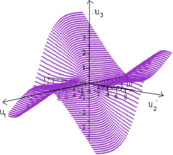
Fig. 1. (a) The phase space of (1) with A 1 = A 2 = 1;

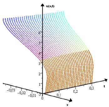
b)

v 1(0) = - 0 , 01 ,v 2(0) = - 0 , 01 ,v 3(0) = 0 , 02

(b) The solution to (8) with

sums

NN uГ(x,t) = ^ vi(t)

where xi ( x ) = ( Ci ( x ) , Zi ( x )) ^are the eigenfunctions of the Sturm-Liouville problem on the graph. For N = 2 the eigenvalues and eigenfunctions are

T 1 = 0 , x 1 = (cos x, — cos 2 x ) ,

T2 = 1| ,X2 = (cos 7, cos7x — sin7x), 16           4     44

and so we look for the solution in the form

x u 1 (t, x) = v 1 (t) cos x + v2 (t) cos 4,

7 x7 u2(t, x) = —v1(t)cos2x + v2(t)(cos 4— sin 4).

In the case A 1 = 1 and A2 = 4 the hypotheses of claim (ii) of Theorem 1 hold because 0 G a ( L ).

Multiplying (11) by the functions xk f°^r k = 1 , 2, we obtain the system of differential equations

J — 7 v 2( t ) v 2( t ) + 93 v i( t ) v 2( t ) + 33 v 3( t ) + 963 v 1 ( t ) + 30 v ₂( t ) + 4 v 3( t ) = 0 , [ 142 v ₂( t ) + 136 v₂( t ) — 0 , 2 v 3( t ) + 3 v ₁( t ) + 9 v 2( t ) v 2 ( t ) + 1 v ₁( t ) v 2 ( t ) + 5 v 3( t )=0 .

Figure 2.a depicts the phase space of (10).

Let us solve the Showalter-Sidorov problem for (10) with the data v 1(0) = — 0, 01, v 2(0) = — 0, 01, a nd v 3(0) = 0, 02, which corresponds to the initial condition u 1(x, 0) = — 0, 01 — 0, 01 cos x + 0, 02 cos( ^), u2(x, 0) = — 0, 01 — 0, 01 cosx — 0, 02 sin(4)

Table 2

The numerical solution to (10) with the initial condition u 1(0) = — 0 , 032, u 2(0) = 1

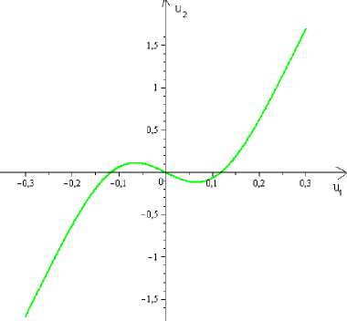
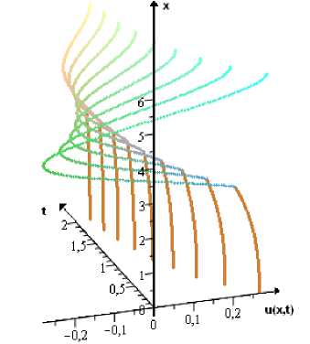
Fig. 2. (a) The phase space of (10) with A 1 = 1 and A2 = 4; (b) The solution to (10) with u 1(0) = — 0 , 032. u2(0) = 1. aiid A 1 = 1. A2 =4

b)

t u 1( t) u 2( t) 0 —0,0326786 1 0,4 —0,020976 0,65291 0,8 —0,013661 0,428574 1,0 —0,011055 0,347559 1,2 —0,008956 0,281959 1,4 —0,00726 0,228795 1,6 —0,005889 0,185683 1,8 —0,004778 0,150710 2,0 —0,003877 0,122333 for (11). Table 2 lists some values of the solution to (10) in a neighbourhood of the point t = 0, while Figure 2.b depicts its graph.

Example 3. Take the finite oriented graph G with three vertices V 1, V2 a nd V3, and with adjacent edges E 1. of It-ngth 1 1 = n and area, d 1 = 7 of crossstiction. and E2. of length 12 = n and d2 = 1 area, of cross-section.

Consider on Hoff’s equations G with the coefficients A 1 = 1 and A2 = 4:

J ^u 1 t + ^u 1 xxt + ^a 11 ^u 1 + ^a 21 ^{u 3} = ⁰ [ ^{4 u} 2 1 + ^u 2 xxt + ^a 12 ^u 2 + ^a 22 ^u 2 = ⁰ •

(П)

The continuity condition is u 1( n, t ) = u ₂(0 , t ), and the flow balance conditions are 7 u 1 _x (0 , t ) = 0, 7 u 1 _x ( n,t ) = u 2 _x (0 , t ), a nd u 2 _x ( n,t ) = 0. We have to find the numerical solution to the inverse problem with Showalter-Sidorov initial conditions with ф 1 = — 0 , 06,

Ф 2 = - 0 , 6. ф 1 = - 0 , 096. ф 2 = - 0 , 96.

cos x.

_{z х}                         ,     7 x        7 x,

u 1o ( x ) = - 0 , 1 cos x + 0 , 3

u 20 ( x ) = 0 , 1cos2 x + 0 , 3(cos 4— sin 4) .

• Theorem 2 implies that

u 10(0) = 0, 2, u 10(n) = 0, 05(2 + 3 V2) ^ 0, 312, u20(0) = 0,4,   u2o(n) = 0, 1(1 + 3V2) ^ 0, 524, ф 1 = -0, 06, ф2 = -0, 6, ф1 = -0, 096, ф2 = -0, 96. Therefore, 01 = 0, 003579 = 0 and 92 = 0, 024 = 0, so the hypotheses of claim (ii) of Theorem 2 hold. The unknown coefficients a 1 = -0, 295. a2 = -1, 03. в 1 = -0, 134. aiid в2 = -2, 9 are nonzero and of the same sign.

The author is grateful to Georgy Anatolevich Sviridyuk for his support and interest in this work.