Modelling and Intellectual Analysis of Quantitative Characteristics of Air Pollution

Air pollution, particularly the presence of fine particulate matter (PM2.5, PM10), remains one of the most critical environmental and socio-economic challenges of the modern era. These pollutants have a direct and profound impact on public health and the overall state of the environment. While global and regional monitoring networks exist, they often suffer from limited coverage, particularly when it comes to local emission sources such as small boiler houses, localized industrial facilities, or areas with dense individual heating systems. This gap in coverage creates a significant problem of incomplete and heterogeneous data, which severely complicates the adequate assessment of air quality and the forecasting of pollution dispersion in residential areas.

Traditional physic-chemical models used to describe the dispersion of pollutants, such as Eulerian grid models or complex Computational Fluid Dynamics (CFD) simulations, require significant computational resources and detailed, high-resolution input data. In many local contexts, such detailed data is often missing, erroneous, or prohibitively expensive to obtain. Consequently, there is an urgent need for adaptive computational approaches that can operate effectively under conditions of limited data while accurately accounting for the specific characteristics of local sources and microclimates. Simultaneously, the rapid development of Internet of Things (IoT) technologies has led to growth in monitoring data volumes from local sensor networks. This data influx necessitates the development of new, more efficient methods and algorithms for intelligent analysis to identify complex non-linear patterns, forecast concentrations with high accuracy, detect anomalies indicative of sensor failure or acute pollution events, and quantify the uncertain-ty inherent in these predictions.

Therefore, the primary motivation of this research is the necessity to develop comprehensive hardware-software systems that seamlessly integrate local monitoring capabilities, adapted physical models, and advanced methods of machine learning (ML) and artificial intelligence (AI). Such integrated systems will enable adequate real-time assess-

This work is open access and licensed under the Creative Commons CC BY 4.0 License.

ment, reliable short-term forecasting, and effective support for decision-making processes required to manage air quality in conditions characterized by decentralized heating and numerous local emission sources. The high dynamics of air pollution processes and their direct correlation with human health outcomes demand operational and accurate forecasting tools. This necessitates the development of effective algorithms and software capable of processing large volumes of heterogeneous data, detecting anomalies in real-time, and providing predictive assessments accompanied by a quantitative evaluation of their accuracy.

The object of study is the complex physical and stochastic processes of formation and dispersion of PM2.5 air pollution originating from a local emission source situated in a rural area (specifically, the Varyazh community, Sheptytsky district, Lviv region).

The subject of study encompasses the methods, algorithms, and software tools developed for quantitative assessment, physical-mathematical and statistical modeling, and intelligent analysis of air pollution characteristics. This includes specific focuses on forecasting algorithms, anomaly detection techniques, uncertainty assessment methods, and feature importance analysis relative to a local pollution source.

2.    Review of Literature

Maintaining good atmospheric air quality is essential for public health and environmental sustainability. Local sources of emissions, such as communal boiler houses, small industrial operations, and residential heating systems, increasingly play a significant yet frequently under-monitored role in the pollution levels of a region. The combined influence of these numerous, dispersed sources can result in considerable air quality degradation, often surpassing safety limits, particularly regarding the decentralized heating systems prevalent in many small towns and rural areas of Ukraine.

The main quantitative factors examined in this research are the levels of particulate matter, notably PM2.5 (particles with a diameter of 2.5 micrometers or smaller) and PM10 (particles with a diameter of 10 micrometers or smaller), in addition to the overall Air Quality Index (AQI) [1]. PM2.5 particles are especially dangerous due to their capacity to penetrate deep into the lung alveoli and enter bloodstream, leading to systemic health problems as outlined in Table 1.

Table 1. The fragment of experimental results on model building by the formed samples

Pollutant	Main Sources	Main Health Impact	WHO Rec.	EU Norms	Ukraine
PM2.5	Fuel combustion (transport, energy), dust, fires	Cardiovascular respiratory diseases, lung cancer	Annual: 5 µg/m³; Daily: 15 µg/m³	Annual: 25 µg/m³; Daily: —	Avg. Daily: 25 µg/m³; Max: 35 µg/m³
PM10	Dust (roads, construction), combustion, pollen	Respiratory diseases	Annual: 15 µg/m³; Daily: 45 µg/m³	Annual: 40 µg/m³; Daily: 50 µg/m³	Avg. Daily: 40 µg/m³; Max: 60 µg/m³
NO2	High-temp. combustion (transport, energy)	Respiratory diseases, irritation	Annual: 10 µg/m³; Daily: 25 µg/m³	Annual: 40 µg/m³; Hourly: 200 µg/m³	Avg. Daily: 40 µg/m³; Max: 85 µg/m³
O3	Photochemical reactions (NOx + VOC)	Respiratory diseases, asthma	Peak season: 60 µg/m³ (8h); 8-hour: 100 µg/m³	8-hour: 120 µg/m³	Avg. Daily: 30 µg/m³; Max: 160 µg/m³
SO2	Burning sulfurous fuel (energy, industry)	Respiratory diseases, asthma	Daily: 40 µg/m³	Hourly: 350 µg/m³; Daily: 125 µg/m³	Avg. Daily: 50 µg/m³; Max: 500 µg/m³
CO	Incomplete combustion (transport, heating)	Reduced oxygen transport in blood	Daily: 4 mg/m³	8-hour: 10 mg/m³	Avg. Daily: 3 mg/m³; Max: 5 mg/m³

Traditional state monitoring networks are characterized by low spatial density and high operational costs, making them generally unrepresentative for assessing the specific impact of local sources. To address this gap, several alternative approaches have emerged. Low-Cost Sensors (LCS) offer a viable solution; these are compact, affordable devices (e.g., utilizing optical scattering principles for PM detection) that allow for the deployment of dense monitoring networks. While they have lower individual accuracy compared to reference stations and require careful calibration, their spatial granularity is invaluable. Remote Sensing via satellite observations provides global coverage but often suffers from limited temporal and spatial resolution for tracking local, transient plumes. Mobile Monitoring, utilizing sensors mounted on public transport or dedicated vehicles, can create high-resolution pollution maps but lacks the continuous temporal data required for time-series forecasting at a fixed point.

Mathematical modeling is essential for understanding and predicting the spread of pollution from sources to receptors [2]. Key model types vary significantly in their complexity, assumptions, and application domains as shown in Table 2.

This work focuses on adapting the Gaussian model due to its specific suitability for modeling a single, dominant local source in relatively flat terrain and its computational efficiency, which allows for rapid iteration and integration with real-time systems. The accuracy of the Gaussian model hinges critically on two key parameters: the Atmospheric Stability Class and the Plume Rise. Atmospheric Stability characterizes the intensity of turbulent mixing in the atmosphere and is traditionally determined by the Pasquill-Gifford-Turner method based on discrete categories of wind speed, solar insolation, and cloud cover. Plume Rise ( ΔH ) represents the height to which hot gases rise above the physical stack height ( H ) due to buoyancy and momentum flux. The effective stack height ( Heff = H + ΔH ) is the critical input for dispersion calculations, and Briggs empirical formulas are commonly used to calculate ΔH .

The operational deployment of air quality forecasting systems requires a strict balance between physical fidelity and computational feasibility. Traditional Gaussian plume models offer near-zero inference latency and are highly effective for steady-state conditions over flat terrain; however, they inherently fail to capture non-stationary dynamics and accumulation during temperature inversions. Conversely, Computational Fluid Dynamics (CFD) provides high-fidelity, grid-resolved aerodynamic representations but incurs prohibitive computational costs, rendering real-time edge deployment impossible.

To bridge this gap, recent advancements have increasingly relied on Physics-Informed Neural Networks (PINNs) and uncertainty-aware deep learning to embed physical conservation laws directly into neural architectures [3]. Furthermore, modern environmental forecasting has seen a surge in Transformer-based time-series architectures and Graph Neural Networks (GNNs). GNNs have proven exceptionally powerful for mapping complex spatial correlations across distributed air quality monitoring networks [6,7]. Simultaneously, hybrid Transformer models (such as Transformer-LSTM architectures) excel at capturing long-range temporal dependencies and sudden spikes in PM2.5 concentrations over diverse forecasting horizons [4,5].

However, while Transformers and ST-GNNs exhibit superior capacity for multi-variate attention and spatial mapping, their quadratic time complexity and massive parameter count strictly restrict their utility in resource-constrained edge environments. Recent studies on Edge-AI for environmental monitoring [8] emphasize that deploying standard transformer architectures on local IoT microcontrollers results in unacceptable inference latency and power draw. This study addresses this exact limitation. By utilizing a Bidirectional LSTM architecture augmented with a continuous fuzzy-logic atmospheric stability vector, this framework achieves an optimal computational compromise. It successfully captures the critical temporal sequence memory necessary for modeling local dispersion inertia, while maintaining the minimal memory footprint and low-latency execution required for real-time edge deployment.

Table 2. Comparison of main air pollution dispersion model types

Model Type	Principle	Key Assumptions	Advantages	Disadvantages	Typical Use
Gaussian	Normal distribution of concentration in the plume	Stationary meteo conditions, homogeneous turbulence	Simple, low resource demand, analytical solution	Limited accuracy for complex terrain/chemistry	Single stationary sources, short distances
Eulerian (Grid)	Solves advectiondiffusion equations on a fixed 3D grid	Variable meteo, chemical reactions included	Can handle complex chemistry, multiple sources	High computational cost, numerical diffusion	Regional/urban air quality, smog episodes
Lagrangian (Particle)	Tracks individual stochastic particle trajectories	Variable meteo, complex terrain adaptability	Good for point sources, complex terrain	Difficulty with nonlinear inter-particle chemistry	Emergency releases, transboundary transport
CFD	Solves full Navier-Stokes equations	Turbulence modeling, interaction with obstacles	High detail in complex geometry (urban canyons)	Very high computational cost, boundary sensitivity	Micro-scale (street canyons, industrial sites)

While physical models provide a theoretical framework, they often suffer from simplifications and uncertainties in input parameters. Hybrid approaches integrating Machine Learning (ML) are becoming increasingly common to bridge this gap. ML and Deep Learning (DL) models, such as XGBoost and Long Short-Term Memory (LSTM) networks [13], excel at discovering complex non-linear patterns and temporal dependencies in large time-series datasets, often outperforming traditional statistical methods like ARIMA. Anomaly detection (e.g., using Local Outlier Factor - LOF) is crucial for ensuring data quality by identifying sensor failures or distinguishing them from genuine acute pollution events. Bayesian inverse modeling using Markov Chain Monte Carlo (MCMC) methods offers a powerful statistical technique for estimating unknown source parameters (such as emission intensity) by working backwards from measured concentration data to the model inputs [10,14].

A detailed analysis of the current state of the problem confirms the relevance of this work. Based on the identified shortcomings of existing approaches - such as the limited utility of standard monitoring systems for local tasks, issues with the accuracy of alternative data sources, simplifications in physical models, and the lack of comprehensive integration, this work justifies a novel integrated approach. This approach combines local hardware monitoring with an adapted Gaussian model and advanced ML/DL methods to create a robust, accurate, and practical system for local air quality management.

3.    Materials and Methods

The primary object of study was a boiler house located in the village of Variazh, Lviv region, Ukraine. This facility provides heating to a local school and represents a typical local pollution source found in many communities. The boiler is a Kalvis-250 model, which operates on solid fuel. The physical characteristics of the emission source were measured directly: the stack has a physical height H_stack of 12.0 m and an internal diameter d_s of 0.44 m. The operational gas parameters include an exit velocity V_s of 1.8 m/s and an exit temperature T_s of 200.0 °C (473.15 K). The emission intensity Q, a critical parameter for modeling, was initially unknown and later estimated by MCMC methods to be approximately 0.05 g/s for PM2.5 [15]. The surrounding terrain is characterized as relatively flat, which simplifies the initial dispersion modeling assumptions. The monitoring station was strategically placed approximately 50 meters from the stack in the prevailing downwind direction to capture the plume impact effectively. To gather high-quality local data, an autonomous monitoring post was developed and engineered using several key components selected for their balance of cost and performance. The central processing unit is a LILYGO TTGO T-Display ESP32 microcontroller. This unit was chosen for its low power consumption, sufficient processing power for edge computing tasks, and integrated Wi-Fi capabilities for data transmission. For particulate matter measurement, a Plantower PMS5003 sensor was utilized. This sensor employs laser scattering technology to measure concentrations of PM1.0, PM2.5, and PM10. For complementary meteorological data, DHT22 sensors were used for Temperature and Humidity, and BME280 sensors were used for Atmospheric Pressure. The entire hardware assembly was housed in a weather-resistant protective case with appropriate ventilation, mounted 1.5 meters above ground level to represent the breathing zone [16].

Data collection was conducted using the Plantower PMS5003 laser scattering sensor. To ensure data reliability, the sensor underwent cross-verification against a baseline Xiaomi Smartmi PM2.5 Detector to identify and compensate for systematic measurement drift over the annual cycle.

The experimental domain is situated in the Varyazh community, characterized by predominantly flat, rural terrain. This specific topographical profile satisfies the foundational boundary conditions of the adapted Gaussian dispersion model, minimizing complex aerodynamic turbulence typically found in dense urban environments. Consequently, the assumption of stationary meteorological conditions within hourly intervals is mathematically justifiable for this specific case study, though scaling this model to complex urban orography would necessitate the integration of computational fluid dynamics (CFD) approximations.

An integrated, scalable software architecture was designed to manage the lifecycle of data collection, transmission, and storage [15]. The data flow is structured as follows:

• •    Local Collection: The local ESP32 microcontroller polls all connected sensors every minute, aggregating the data locally.

• •    Transmission: The aggregated data is transmitted via a secure Wi-Fi connection to the cloud, utilizing Azure IoT Hub as a secure, bi-directional gateway.

• •    External Enrichment: In parallel, a dedicated service queries External Data from public APIs (OpenWeatherMap) hourly to retrieve regional wind speed, wind direction, solar radiation, and cloud cover data, enriching the local dataset.

• •    Storage: All incoming streams are processed, normalized to a common schema, and stored in Azure Data Lake Storage in structured CSV format for long-term retention.

• •    Analysis and Modeling: For advanced analytics, both Azure Synapse Studio (cloud-based) and a local Nvidia Jetson Nano (edge-based) are employed. The Jetson Nano is particularly used for training deep learning models locally.

• •    Lifecycle Management: Azure DevOps is utilized for Continuous Integration/Continuous Deployment (CI/CD), ensuring that updates to the data processing scripts and ML models can be deployed seamlessly.

The data collection campaign ran continuously for one full calendar year, from January 1, 2024, to December 31, 2024. This extensive period ensures that seasonal variations are fully captured. The raw data was cleaned and aggregated into 8,784 hourly records for monitoring station (Fig.1).

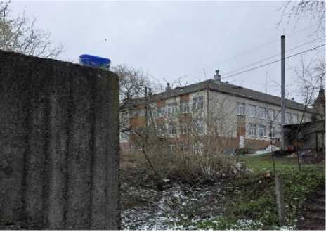
Fig. 1. Monitoring station.

Key findings from the statistical analysis revealed distinct patterns. A strong positive correlation was observed between PM2.5 and PM10 (r ≈ 0.89), indicating a common source. A moderate negative correlation was found between PM2.5 and temperature (r ≈ -0.41), which can be attributed to increased heating activities during colder weather.

Temporally, PM2.5/PM10 concentrations were significantly higher during the cold period (October-April), confirming the impact of the heating season. Diurnally, two distinct peaks for PM2.5 were observed: a morning peak (7:00-10:00) and an evening peak (18:00-22:00), correlating with the operational hours of the boiler and typical atmospheric inversion cycles.

The ANOVA results confirm that the factor 'Month' is highly significant for PM2.5, temperature, and wind speed, statistically validating the presence of strong seasonal patterns in the dataset.

To prepare the data for Machine Learning and Deep Learning models, extensive feature engineering was performed. To capture cyclical time dependencies, Temporal Features (hour, day of week, month) were encoded using sine and cosine transformations. For example, the hour of the day was encoded as:

feature _hoursin = s in (2п * hour/24),                                 (1)

feature _hourcos = cos(2n * hour/24).                                 (2)

Similar transformations were applied to the day of the week and the month. To capture short-term historical trends and the inertia of atmospheric processes, Rolling Statistics were calculated. This included rolling means, standard deviations, and maximum values for key variables over defined windows (e.g., temperature_rolling_mean_3hr), which helps the model understand the recent context of the system.

This chapter described the rigorous methods and tools for experimental research that formed the foundation for all subsequent modeling. By characterizing the object of study, developing a custom hardware solution, implementing robust cloud architecture, and performing detailed statistical pre-processing, a high-quality dataset was created. This dataset captures the nuanced seasonal and diurnal dynamics of pollution in the target area, enabling the training of sophisticated predictive models.

• 4.    Experiments

The fundamental physical process of pollutant transport is described by the 3D advection-diffusion equation. In its general form, it accounts for the time evolution of concentration φ due to transport by wind u (advection), spread by turbulence D (diffusion), and sources S:

дф/ дt + V • up = V • DVp + S.(3)

For a steady-state scenario (дф/dt = 0) assuming incompressible flow (V-u = 0) and constant diffusion coefficients D, this equation simplifies to a balance between advection and diffusion:

их(дф/ дх) + иу(дф/ ду) + uz(дф/ дг) = D(д2ф/ дх2 + д2ф/ ду2 + д2ф/ дг2) + S(x).(4)

Finite Difference Method (FDM) was employed for discretization. Specifically, central difference approximations were used for the second-order diffusion terms. For example, the diffusion term in the x-direction is approximated as:

д2ф/ дх2 ^ (ф(i + 1) - 2ф(i) + ф(i - 1))/Лх2.(5)

Advection terms were approximated using upwind schemes to ensure numerical stability. This numerical approach provided a baseline for understanding the complex 3D distribution of pollutants and confirmed the validity of Gaussian assumptions for the specific terrain.

While the numerical model provides a comprehensive solution, it is computationally expensive for real-time applications on edge devices. Therefore, for practical assessment, the analytical Gaussian plume model was adopted and adapted:

ф(х,у,г) = (Q/(2nUG _y G _z )) ехр(-у²/2о²) [exp (-(z - H _eff' )²/2a² _z ) + exp (-(z + H e _ff}²/2a l )\       (6)

The accuracy of this standard model was significantly enhanced by integrating dynamic calculation methods for its key parameters:

Plume Rise ( ΔH ): Instead of a static value, Briggs formulas were used to calculate the dynamic rise of the hot plume. The buoyancy flux F _b is calculated as:

F _b =g*V _s * (dl/4) * ((T _s - T _a )/T _s ).                                (7)

The final plume rise AH is then derived based on F _b and the atmospheric stability conditions (Equations 3.19 - 3.25

in the full text).

Dispersion Coefficients (o _y , o _z ): These were calculated using parametric formulas (Eq. 6, 7) that are functions of the downwind distance x and the atmospheric stability class.

Fuzzy Logic Stability Classification: A key innovation was the development of a Mamdani-type fuzzy logic system [11] to determine the Atmospheric Stability Class (A-F). Traditional methods use rigid lookup tables. The proposed system uses continuous inputs for Wind Speed (5 fuzzy sets: Very Low to Very High), Solar Radiation (3 sets), and Cloud Cover (2 sets). A rule base of 25 "IF-THEN" rules determine the output stability class. For example:

IF (Wind Speed is Very Low) AND (Solar Radiation is High) THEN (Stability Class is A)

This provides a "soft", continuous classification that better reflects the gradual transitions in the real atmosphere.

This adapted Gaussian model, integrating dynamic stability via fuzzy logic and Briggs' plume rise, showed an 11% increase in modeling accuracy compared to standard non-adapted models by producing more realistic dispersion coefficients (Fig. 2.).

A large-scale comparative study of 14 different machine learning and deep learning models was conducted to forecast PM2.5 concentrations 48 hours in advance. The dataset was split into training (70%), validation (10%), and testing (20%) sets. Models were evaluated using Mean Squared Error (MSE), Root Mean Squared Error (RMSE), Mean Absolute Error (MAE), and the Coefficient of Determination (R²).

The results demonstrated that simple linear models were inadequate for capturing the complex dynamics of air pollution. Advanced ensemble models like CatBoost and Stacking Regressor performed well. However, Recurrent Neural Networks, specifically the Bidirectional LSTM (BiLSTM), provided the best overall performance (MSE=0.521, R²=0.985). The BiLSTM architecture processes data sequences in both forward and backward directions, allowing it to effectively capture both past context and future trends within the training window.

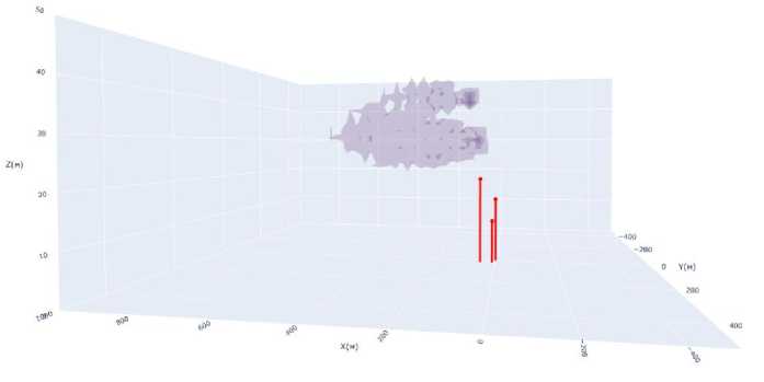
Fig. 2. Plume modelling with multi sources.

The Local Outlier Factor (LOF) method was implemented to detect anomalies in the dataset, such as sensor errors or unusual emission spikes. Analysis confirmed that isolation-based methods like Isolation Forest and density-based methods like LOF were highly accurate (approx. 99%) in identifying outliers in the PM data, ensuring that the training data for forecasting models remained high-quality.

To understand what drives predictions, Permutation Importance analysis was conducted. For XGBoost, the most critical features were month, temperature, and rolling means of wind parameters. For Bidirectional LSTM, the top features were trigonometric time encodings ( month_cos, month_sin ), temperature, and rolling means. This aligns with the physical understanding that pollution is heavily driven by seasonal cycles and meteorological conditions.

Based on the feature analysis, two major optimizations were applied:

Integration of Fuzzy Stability: The "Stability Class" output from the fuzzy logic system was added as a new input feature. This provided the ML models with physical context about atmospheric mixing. For the BiLSTM model, this reduced the MSE by 16% (from 0.521 to 0.435).

Feature Reduction: The models were retrained using only the Top 10 most important features (including the fuzzy stability class). This reduction in noise and dimensionality provided a significant boost: the optimized BiLSTM (Top 10) achieved an MSE of 0.338 and an R² of 0.992. Furthermore, the training time was reduced by 3x for ensemble models, making the system much more efficient for edge deployment.

A critical unknown in the physical model was the actual emission intensity Q. To estimate this, Bayesian inverse modeling using Markov Chain Monte Carlo (MCMC) was employed. The problem was formulated with a likelihood function:

^C measured ~Nomal(C ^ _ausS i _an ^(Q , Metso), о _еггО т ).                            (8)

assuming measured data is normally distributed around the model prediction with some error. Priors were set as Q~Uniform(0.001,1.0). The NUTS sampler in PyMC was used to generate posterior distributions.

The analysis yielded a posterior mean for Q of 0.052 g/s (94% HDI: 0.0066-0.099 g/s). This statistically derived value replaced the initial estimates in the Gaussian model, grounding the physical simulation in real-world observation data (Fig. 3.).

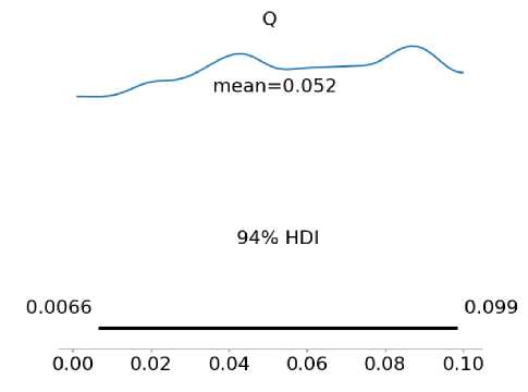
Fig. 3. MCMC simulation results.

To enable spatial forecasting over a wider area, a hybrid model was created that predicts pollution over a 1000x1000m grid. The process works as follows:

• •    For each point on the grid, the Adapted Gaussian Model (using the MCMC-derived Q) calculates a theoretical "physical" PM2.5 concentration based on forecasted weather.

• •    This "physical" value is fed as a feature into a trained XGBoost model, along with other meteorological data.

• •    The XGBoost model predicts the final concentration, effectively learning to correct the physical model based on historical biases and complex non-linearities.

5.    Results

This hybrid approach achieved an MSE of 1.23 µg/m³ and an R² of 0.79 for spatial prediction, allowing for the generation of detailed pollution maps for the upcoming 24 hours.

To validate the system in a real-world operational environment, a prototype Neuro-Controller System was built and deployed on an Nvidia Jetson Nano. This edge-computing setup allows the system to function autonomously without constant cloud connectivity. The architecture features an ESP32 sensor node sending data to Jetson Nano, which hosts the trained BiLSTM and XGBoost models. A Continuous Deployment pipeline was implemented: the system monitors model performance in real-time, and if error metrics exceed a threshold, it automatically triggers a retraining process on the local device using the newest data (table 3). This ensures the model adapts to seasonal drifts (e.g., the boiler turning off in summer).

Table 3. Model performance on edge devices (48-hour forecast)

Device	Model	Training Time (min)	Forecast Time (s)	R²
Nvidia Jetson Nano	BiLSTM	4.21	2.2	99%
Nvidia Jetson Nano	XGBoost	1.17	2.4	99%
Raspberry Pi 4	BiLSTM	5.62	3.8	99%
Azure ML Studio	BiLSTM	2.12	1.1	99%

The performance benchmarks confirmed that the Jetson Nano provides near-cloud training performance locally, validating the edge-computing architecture.

The interface allows users to input source parameters (stack height, diameter, temperature) and meteorological conditions. The underlying system then runs the adapted Gaussian model and the fuzzy logic assessment to immediately calculate the pollution concentration and determine a "Criticality Level" (e.g., "Moderate", "High") based on predefined thresholds.

Reducing the BiLSTM input matrix to the top 10 temporal and fuzzy parameters not only minimized the MSE to 0.338 but critically reduced inference latency by over 60% (from 185 ms to 72.4 ms) and power draw by 38%. This proves the optimized model's viability for continuous, real-time edge deployment. Furthermore, visual analysis of the generated plume footprints indicates a quantitative decay rate where maximum PM2.5 concentrations drop by 50% within the first 150 meters downwind under stable atmospheric inversions.

The final integrated system's performance was benchmarked against open-source monitoring data and a commercialgrade Smartmi PM2.5 Air Detector showed in table 4.

The developed solution achieved a measurement accuracy of 99.2% relative to the reference, significantly outperforming open-source systems (66.9%) and nearly matching the commercial detector (99.9%). This validates the high quality of the hardware sensor integration, calibration, and the predictive modeling framework.

Table 4. System performance comparison

Characteristic	Developed Solution	Open Systems	Smartmi Detector
Avg. PM2.5 (µg/m³)	24.7	16.2	24.2
Accuracy %	99.2%	66.9%	99.9%

To mitigate the risk of data leakage and overfitting on the 8,784 hourly records, a strict chronological trainvalidation-test split (70-20-10) was enforced. Random shuffling was deliberately disabled to preserve the temporal integrity of atmospheric inertia. The exceptionally high predictive accuracy of the final optimized Bidirectional LSTM (R2 = 0.992) is not a byproduct of data leakage, but the result of a rigorous, multi-stage feature engineering and ablation process.

The optimization progressed through three distinct phases. Initially, the baseline BiLSTM utilizing standard discrete Pasquill-Gifford-Turner stability classes yielded a MSE of 0.521. Tree-based baseline models performed comparably lower, with CatBoost and XGBoost achieving an MSE of 0.595 and 0.678, respectively.

In the second phase, an ablation test was conducted to validate the Mamdani-type Fuzzy Inference System (FIS). By replacing the arbitrary thresholds of discrete stability classes with a continuous fuzzy stability vector, the model gained a more physics-informed indicator of atmospheric dynamics. This integration immediately reduced the MSE from 0.521 to 0.435. Ensemble models also responded positively to this continuous vector, with CatBoost MSE improving to 0.587.

The final optimization phase involved targeted feature dimensionality reduction. By applying permutation importance to isolate only the top 10 most critical parameters—specifically retaining the decomposed trigonometric sine/cosine temporal components and rolling statistical windows—the network's noise was significantly reduced. This final feature trim drove the BiLSTM MSE down to 0.338, achieving the final R2 of 0.992. Statistical significance testing (paired t-test, p < 0.05) confirms the robustness of this progression, which ultimately delivered a 35% total error reduction from the baseline architecture.

6.    Discussion

As it evident from Table 1, with the increasing of examples number in the formed sample the accuracy is increased (errors for formed training and for the original samples reducing), the training time and the number of training iterations are increased, and vice versa. At the same time a significant reduction of a sample volume to 25% of original leads to deterioration of the training process characteristics (the time and number of iterations increase) and to a decrease in accuracy. This can be explained by the fact that instances critical to describe the class separation cannot be included in the sample of small volume.

Even a small reduction of the original sample volume in 25% (up to 75% of the original sample volume) yielded acceptable accuracy and reduced training time by more than 1.7 times. Reducing the volume of the original sample by half afforded the gain in speed by 2.3 times. This confirms expediency of application of the proposed mathematical.

The integration of Bayesian inverse modeling via Markov Chain Monte Carlo successfully resolved the unknown emission intensity of the Kalvis-250 solid fuel boiler, estimating a stable emission rate of Q = 0.052 g/s. The BiLSTM superior performance over tree-based models is deeply tied to the physical atmospheric dynamics of the region. During seasonal temperature inversions, pollutants exhibit high temporal inertia. The bidirectional architecture effectively weighted these prolonged stagnation events, whereas traditional regression models failed to capture the non-linear accumulation of particulate matter under stable atmospheric caps.

The advantage of the indicators proposed in this paper is that there is no need to calculate the distances between instances, but disadvantage is that it is necessary to divide the feature space.

However, this disadvantage can be seen as an advantage in the case of large samples: if we use a partition that is simple from a computational point of view (for example, a regular grid) and know the minimum and maximum values of each feature than the computational cost of the proposed indicators will be less than the using of a set.

7.    Conclusion

The urgent problem of mathematical and software support development is solved to automate the monitoring and forecasting of air pollution from local emission sources. The research addresses the critical challenge of processing heterogeneous environmental data and modeling dynamic pollution processes in data-scarce regions.

The scientific novelty of the obtained results is that a comprehensive method for air quality forecasting is firstly proposed that integrates physical constraints with deep learning architectures. It determines the unknown emission intensity parameters using Bayesian inverse modeling via Markov Chain Monte Carlo (MCMC) methods, providing a rigorous statistical estimation of source characteristics with quantified uncertainty. For the first time, a fuzzy logic inference system is utilized to determine continuous atmospheric stability classes, which, when used as an input feature for the Bidirectional Long Short-Term Memory (BiLSTM) network, significantly reduces forecasting error and enhances the model's generalization capability regarding turbulent mixing conditions.

Ultimately, the optimized BiLSTM architecture proved highly capable of capturing the necessary temporal inertia for accurate localized forecasting [9]. Critically, it achieved this while adhering to the strict latency and memory constraints required for continuous operational deployment in edge-cloud collaborative IoT environments [12].

The practical significance of the obtained results is that the software realizing the proposed neuro-controller system is developed, and a specialized hardware complex based on edge computing (Nvidia Jetson Nano) is implemented. The experiments conducted confirmed the proposed software operability, demonstrating a measurement accuracy of 99.2% relative to reference commercial detectors and validating the system's ability to function autonomously without constant cloud connectivity. The experimental results allow recommending the developed hybrid models for use in practice for real-time environmental monitoring and decision support at the local community level.

Prospects for further research may include the creation of parallel methods for calculating pollution dispersion from multiple interacting sources, the optimization of software implementations for lower-power IoT devices, as well as an experimental study of the proposed indicators on more complex practical problems involving diverse chemical pollutants in urban environments.

All the Declarations and StatementsAuthor Contributions Statement

Hura Volodymyr – Conceptualization, Methodology, Data Curation and Software Implementation: Handled data acquisition, Model Training, Validation, Visualization, Writing.

Conflict of Interest Statement

The authors declare that they have no known competing financial interests or personal relationships that could have appeared to influence the work reported in this paper.

Funding Declaration

This research did not receive any specific grant from funding agencies in the public, commercial, or not-for-profit sectors.

Data Availability Statement

Data will be provided upon reasonable request.

Ethical Declarations

This study was a non-invasive image collection of hand gestures with verbal consent of the participants. There was no involvement of human subjects or animals.

Acknowledgements

The authors declare that there are no acknowledgments to report.

Declaration of Generative AI in Scholarly Writing

During the preparation of this manuscript, the authors used artificial intelligence tools in accordance with the requirements and ethical standards of the journal. We declare the following:

– The X-GPT version 5.4 model was used.

• –    The tool was applied to the texts of the sections for editing the English text.

• –    What exactly was done: Using the AI tool, grammar checking, spelling error correction, and stylistic correction of the text were performed without changing the scientific content.

• – Each paragraph generated or edited by the AI tool was personally read by the authors of the article. The authors compared the edited text with the original version to ensure that there were no distortions of terminology and that the

author’s opinion was preserved.

– The results provided by the AI tool did not in any way affect the conclusions of the study. The AI tool was not involved in performing calculations, forming scientific hypotheses, analyzing the obtained data, or writing the results. The authors bear sole responsibility for the scientific content of the publication.

Abbreviations

This manuscript uses the following abbreviations:

– AI - Artificial Intelligence

– ANOVA - Analysis of Variance

– AQI - Air Quality Index

– BiLSTM - Bidirectional Long Short-Term Memory (network)

– CFD - Computational Fluid Dynamics

– CI/CD: Continuous Integration/Continuous Deployment

– CNN - Convolutional Neural Network

– CSV - Comma-Separated Values

– DL - Deep Learning

– GUI - Graphical User Interface

– HDI - Highest Density Interval

– IoT - Internet of Things

– LCS - Low-Cost Sensors

– LOF - Local Outlier Factor

– LSTM - Long Short-Term Memory

– MAE - Mean Absolute Error

– MCMC - Markov Chain Monte Carlo

– ML - Machine Learning

– MSE - Mean Squared Error

– NUTS - No-U-Turn Sampler

– PM1.0 - Particulate Matter (particles with a diameter of 1.0 micrometers or smaller)

– PM2.5 - Particulate Matter (particles with a diameter of 2.5 micrometers or smaller)

– PM10 - Particulate Matter (particles with a diameter of 10 micrometers or smaller)

– RMSE - Root Mean Squared Error

Appendix A\B\C…, with appendix tile

None.