Performance Evaluation of Bagging and Boosting- Based Ensemble Learning Models for Clinical Liver Disease Prediction Using the LDPD Dataset

The liver plays a crucial role in maintaining overall health and metabolic balance. It is also considered one of the most vital organs responsible for producing essential compounds, managing waste, removing damaged cells, aiding digestion through bile production, and detoxifying harmful substances. Viruses like hepatitis (A, B, and C), excessive alcohol use, and toxin exposure are common causes of liver damage. These can lead to diseases such as hepatitis, cirrhosis, liver tumors, and liver cancer, with cirrhosis being a leading cause of death worldwide [1]. Liver disease causes around 2 million deaths each year worldwide, including 1 million due to complications of cirrhosis. Globally, cirrhosis is the 11th leading cause of death, while liver cancer ranks 16th. Combined, these conditions contribute to 3.5% of all deaths worldwide [2]. Diagnosing liver disease in its early stages is often challenging, as symptoms can be subtle or absent, leaving many individuals unaware of their condition until significant liver damage has occurred. Early diagnosis is critical for effective treatment and improving health outcomes [3]. With the exponential growth of healthcare data, traditional Machine Learning (ML) methods often struggle to handle the vast volume and complexity of information required for accurate disease prediction. Ensemble learning solves these challenges by combining different ML algorithms into a single robust model to improve accuracy, reliability, and performance, especially for predicting liver diseases compared to standalone models [4]. Several ensemble learning strategies like bagging, boosting, voting, and stacking enhance machine learning performance [5, 6]. The choice of the most suitable model depends on factors such as the particular problem to be solved, the characteristics of the dataset (e.g., size, quality, and distribution), and the computational resources available. In the bagging (bootstrap aggregating) method, multiple subsets are generated from the original dataset with random sampling with replacement. Then a separate base model (typically weak learners) is trained on each subset of the data independently and randomly. Finally, a majority vote is taken from the predictions of all base models to do a classification task. The main advantage of bagging approach is that it is less prone to overfitting than individual models. The Boosting algorithm is a prominent ensemble ML approach developed by Freund and Schapire [7] that

This work is open access and licensed under the Creative Commons CC BY 4.0 License.

combines the predictions of multiple weak learners to create a strong learner. The main idea is to train weak models sequentially, with each model addressing the errors made by its predecessor which improves accuracy and overall prediction performance.

This paper aims to determine a comparative analysis of several ensemble techniques for liver disease prediction with improved accuracy. The main contributions of this paper are as follows:

• i.    An exploratory data analysis along with data preprocessing, normalization and standardization are considered to improve the dataset's quality for experimental use.

• ii.    The effect of features on liver disease prediction is explored.

• iii.    Three bagging and five boosting algorithms are applied to build the prediction model.

• iv.    A comprehensive analysis of bagging and boosting algorithms is performed using diverse performance metrics. v. The proposed model's best performance is compared with other recent studies.

• 2.    Literature Review

• 3.    Research Methodology

The rest of the paper is structured as follows: Section 2 provides related works. The methodology and dataset pertaining to liver disease prediction are elaborated upon in Section 3. Experimental analysis and discussion are presented in Section 4. Finally, Section 5 concludes the paper with a summary of findings and outlines future research directions.

Ghosh et. Al. [8] analyzed the Indian Liver Patient Dataset (ILPD) and presented a comparative analysis of machine learning models for liver disease prediction. They evaluated the models using different training sizes, ranging from 50% to 90% of the dataset. Interestingly, their findings revealed that most algorithms, except AdaBoost, achieved their peak performance at a training size of 80%. Among the evaluated models, the best performance (accuracy: 83.76%) is achieved with RF classifier. Authors of [9] proposed the Tree-Structured Parzen Estimator (TPE) method with different ML algorithms (DT, RF, ETC, LightGBM, and Adaboost) to predict LD. To address the class imbalance problem, they used up sampling process and min-max normalization to scale the dataset as a pre-processing step. It was found that ETC with the TPE approach performed the best with an accuracy of 95.8%. Ganie et. al. [10] uses ILPD and LDPD dataset to predict liver disease utilizing different boosting algorithms like Gradient Boosting (GB), AdaBoost, LogitBoost, SGBoost, XGBoost, LightGBM, and CatBoost. They applied random and grid search approaches to tune model hyperparameters to obtain the best possible outcomes. The analysis of feature importance, based on F-scores, revealed that for both datasets Direct Bilirubin (DB), Alkaline Phosphatase (AP), Alanine Aminotransferase (ALA), and Aspartate Aminotransferase (ASA) are the most significant factors influencing the prediction of liver disease. Conversely, the demographic parameters (Gender and Age) are the least significant factors in the prediction outcomes. For the ILPD and LDPD datasets, GB classifier outperformed others by achieving an accuracy of 98.29% and 98.80% respectively. The authors of [11] evaluated various ensemble learning approaches, including bagging (RF, ETC, Bagged DT), boosting (XGBoost, LightGBM, GB), and voting algorithms (Logistic Regression, DT, Support Vector Machine) to enhance liver disease prediction on LDPD dataset. They incorporated data sampling, standardization, normalization, hyperparameter tuning, and feature selection as auxiliary methods to optimize model performance. Their experimental analysis demonstrated that GB, RF, and the voting classifier achieved the highest accuracy levels of 98.80%, 90.99%, and 84.04%, respectively, representing the top-performing boosting and bagging algorithms. BULUCU et. al. [12] predicted liver disease from machine learning based bagging and boosting ensemble algorithms where clinical datasets were collected from the University of California, Irvine (UCI) data repository. Bagging algorithms like RF, J48 and boosting algorithms like AdaBoost, GB and LightGBM were used. To address the uneven distribution in the original dataset, the Synthetic Minority Over-sampling Technique (SMOTE) technique was applied for data balancing. Among the models, the LightGBM algorithm achieved the highest accuracy of 98.8% using 10-fold cross-validation.

An optimized approach for liver disease prediction was introduced in [13] using the SMOTE integrated supervised learning model. The authors employed KMeans SMOTE, an enhanced version of traditional SMOTE, to generate higher-quality synthetic samples, particularly for complex datasets with class imbalance issues. The study evaluated the performance of K-Nearest Neighbor (KNN) and RF classifiers and found superior results (accuracy 97.60%) compared to KNN.

Feature integration strategy based on Principle Component Analysis (PCA), Linear Discriminant Analysis (LDA) and Factor Analysis (FA) with ML for chronic liver disease prediction was developed in [14] to mitigate the challenges known as the curse of dimensionality [15]. Later on, random sampling was used to reduce bias and overfitting. They also incorporate several ML classifiers such as LR, Support Vector Machine (SVM), KNN, Multilayer Perceptron (MLP) and ensemble voting. Their experimental findings suggest that their proposed method achieved 0.10-18.5% better results than the existing studies. Sreejith et al. [16] used ILPD, Thoracic Surgery (TSD), and Pima Indian Diabetes (PID) datasets for clinical data classification using the class balancing SMOTE (enhanced using Orchard's algorithm, OSMOTE) and the Chaotic Multi-Verse Optimization (CMVO) evolutionary feature selection approach. Without applying OSMOTE and CMVO-based feature selection, they achieved a 69.43% accuracy rate on the ILPD dataset using RF classifier. The accuracy increased to 82.62% when OSMOTE was used without CMVO-based feature selection. An accuracy of 82.46% was obtained by combining OSMOTE with CMVO-based feature selection. P. Kumar et al. [17] focused on the three real world imbalance liver datasets BUPA, ILPD from UCI and MPRLPD to classify liver patients more accurately using a 10-fold cross-validation technique. To diagnose liver patients’ authors incorporated neighbor-weighted KNN (NWKNN), fuzzy-neighbor-weighted KNN, and variable-neighbor-weighted fuzzy KNN classifiers (Variable-NWFKNN). The dataset was balanced using Tomek Link and Redundancy-based Under-Sampling (TR-RUS) technology which improved the accuracy of their proposed Variable-NWFKNN classifier to 78.46% for BUPA dataset, 78.46% for ILPD dataset and 95.79% for MPRLPD dataset. A comparative analysis of ML models (Naïve Bayes, Logistic Regression, linear and nonlinear SVM, J48, Random Tree, and Reduced Error Pruning Tree) and ensemble methods (bagging, RF, Rotation Forest, AdaBoostM1, voting, stacking, MLP, and KNN) was conducted in [18] for chronic liver disease prediction. Their findings suggest that among other models voting classifier obtained the highest performance (accuracy 80.1%) with 10fold cross validation after applying SMOTE based data balancing algorithm. Table 1 presents the summary of the existing works.

Table 1. Summary of existing works

Ref.	Method	Preprocessing	Feature Selection / Optimization	Classifier	Accuracy (%)	Limitation
[8]	Comparative ML analysis on ILPD	Different traintest splits (50%-90%)	-	Logistic Regression, RF, XGBoost, SVM, AdaBoost, K-NN, and DT	83.76 (RF)	Limited predictive performance
[9]	TPE-based liver disease prediction on ILPD	Upsampling, Min-Max normalization	Tree-Structured Parzen Estimator (TPE) hyperparameter optimization	TPE with DT, RF, ETC, LightGBM and AdaBoost	95.80 (ETC)	Evaluated only on ILPD, limiting generalizability
[10]	Boosting-based liver disease prediction on ILPD and LDPD	-	Random Search, Grid Search, Feature importance analysis	GB, AdaBoost, LogitBoost, SGBoost, XGBoost, LightGBM, and CatBoost.	98.80 (GB, LDPD) 98.29 (GB, ILPD)	Considered only boosting algorithms
[12]	Bagging and boosting ensemble learning	SMOTE data balancing	-	RF, J48, AdaBoost, GB, LightGBM	98.80 (LightGBM)	Limited feature analysis and interpretability discussion
[13]	SMOTE-integrated supervised learning model	KMeans-SMOTE oversampling	Optimized synthetic sample generation	KNN, RF	97.60	Evaluated a limited number of classifiers
[16]	Clinical data classification using OSMOTE and CMVO	OSMOTE data balancing	CMVO evolutionary feature selection	RF	82.62	Lower performance on liver disease prediction tasks.
[17]	Liver disease prediction on imbalanced datasets	TR-RUS data balancing	-	NWKNN, Fuzzy- NWKNN, Variable-NWFKNN	95.79 (MPRLPD)	Focused mainly on KNN-based methods

Fig. 1. shows the workflow of our research. We have performed exploratory data analysis and data preprocessing steps to find and replace the missing values. Furthermore, we have also detected the outlier or noisy data and removed it from the dataset. Afterward, normalization was applied to scale the data, followed by feature ranking to assess feature importance. To build the learning model we used eight different ensemble models and compared their performance based on diverse performance metrics.

3.1.    Bagging Algorithms

In our work, we have used Random Forest, Extra Trees Classifier and Bagged Decision Tree algorithms as a bagging method.

• 3.1.1.    Random Forest (RF)

• 3.1.2.    Extra Trees Classifier (ETC)

• 3.1.3.    Bagged Decision Tree (Bagged DT)

3.2.    Booting Algorithms

• 3.2.1.    Adaptive Boosting (AdaBoost)

Random forest is a robust and versatile machine learning algorithm where multiple decision trees are constructed during training and combined their predictions to enhance accuracy and stability. It operates by creating random bootstrapped sampling with replacement to generate subsets of data and randomly selecting features at each split; therefore, it introduces diversity among the trees, reducing overfitting and improved generalization. For classification tasks, it predicts by majority voting across the trees, while in regression tasks, it computes the average of their outputs. Despite its computational cost due to the training of multiple deep trees, RF is immune to noise and outliers and performs well even with unbalanced or partially missing data.

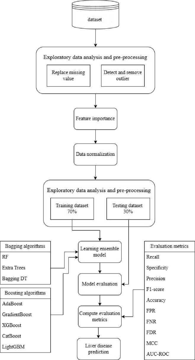
Fig. 1. Architecture of our methodology

Extra Trees Classifier is another ML approach and similar to RF that trains multiple decisions and combines their results to make predictions. The main difference is in how they create these decision trees. RF uses a bagging , which selects different subsets of the training data for each tree whereas ETC trains decision trees on bootstrapped samples but selects split points randomly. This randomness gives ETC slightly higher bias (less precise predictions) but lower variance (more consistent results) [19].

Bagged Decision Tree is a powerful ensemble method to improve the performance and stability of unstable classification methods like decision trees, especially when the base decision tree model suffers from high variance [20]. Bagged DT, generates multiple bootstrap samples from the original dataset and trains multiple trees on these different datasets then combines (majority voting) their results to make a final prediction.

In our work, we have used Adaptive Boosting, Gradient Boosting, Xtreme Gradient Boosting, Categorial Boosting and Light Gradient Boosting Machine as a boosting method.

AdaBoost is an iterative machine learning algorithm that creates a strong classifier by combining multiple weak classifiers [21]. It repeatedly trains a weak learning model (decision tree stumps) on the same dataset while dynamically modifying the weights of both training samples and weak classifiers to improve overall performance. Misclassified samples have greater weights in subsequent iterations, increasing their influence on the learning process. Meanwhile, weak classifiers with lower error rates are prioritized, contributing more significantly to the final model [22].

• 3.2.2.    Gradient Boosting (GradientBoost)

• 3.2.3.    Xtreme Gradient Boosting (XGBoost)

• 3.2.4.    Categorial Boosting (CatBoost)

• 3.2.5.    Light Gradient Boosting Machine (LightGBM)

3.3.    Hyperparameter Tuning

Gradient Boosting combines gradient descent and boosting to iteratively reduce the loss function and build a predictive model. It employs decision trees as weak learners, with each subsequent tree focusing on correcting the errors of the previous one. The method refines predictions toward the target values by calculating residuals (the gap between actual and anticipated values) and aligning weak learners to them. GradientBoost, unlike RF, generates trees sequentially rather than independently making it more computationally intensive but typically more accurate [23].

CatBoost is an implementation of gradient boosting algorithm, designed for classification, regression and ranking tasks. It is specially optimized for categorical features, using order encoding and target-based statistics to minimize preprocessing. CatBoost reduces overfitting by shuffling features and calculating average label values for categorical features during training. Key features of CatBoost include feature combination, which greedily combines features to generate more powerful ones, and fighting gradient bias, which uses a modified version of gradient-based decision trees to build the tree structure and traditional methods for setting leaf values [25].

LightGBM is an optimized gradient boosting algorithm developed by Guolin Ke et al. that focuses on computational efficiency while maintaining high accuracy to handle large datasets effectively. Unlike other gradient boosting algorithms, it employs the leaf-wise (best-first) tree technique strategy to grow the leaf, which reduces more loss and improves accuracy while growing on the same leaf. The important features of LightGBM include Gradient-based One-side Sampling (GOSS) , which speeds up the best split point finding by focusing on high-gradient data, and Exclusive Feature Bundling (EFB) , which speeds up split finding by considering only data points with higher gradients, and EFB, which groups mutually exclusive features to reduce computational complexity and makes the overall training speed of LightGBM 20 times faster than other traditional gradient boosting decision trees [26].

We optimize our bagging and boosting algorithms performance by tuning the hyperparameters: random state and n_estimators of both bagging and boosting algorithms while keeping all other hyperparameters at their default values to avoid introducing optimization bias toward particular models. Table 2 presents the hyperparameter tuning values.

Table 2. List of hyperparameter values chosen by this research

Hyperparameter Value	RF	ETC	Bagged DT	AdaBoost	GradientBoost	XGBoost	CatBoost	LightGBM
Random state	42	42	42	none	45	42	45	42
n_estimators	5000	5000	5000	6000	6000	1000	6000	4000

3.4.    Datasets

We have collected the LDPD from [27]. Table 3 presents the dataset distribution, while Table 4 provides details about the dataset attributes, including their mean and standard deviation values.

Table 3. Dataset description

Dataset	Total Records	Liver Patients	Not Liver Patients	Male	Female
LDPD	30691	21917	8774	21986	7803

Table 4. Attributes list

Serial No.	Attribute	No. of Missing Values	Data Type	Measurement Unit	Range	Mean	Standard Deviations
1	Age (AG)	2	Numeric	Years	4-90	44.1072	15.9810
2	Gender (GN)	0	Nominal	N/A	N/A	N/A	N/A
3	Total Bilirubin (TB)	648	Real Number	mg/dl	0.4-75	3.3703	6.2555
4	Direct Bilirubin (DB)	561	Real Number	mg/dl	0.1-19.7	1.5280	2.8695
5	Alkaline Phosphatase (AP)	796	Numeric	U/L	63-2110	289.0753	238.5375
6	Alanine Aminotransferase (ALA)	538	Numeric	U/L	10-2000	81.4886	182.1588
7	Aspartate Aminotransferase (ASA)	462	Numeric	U/L	10-4929	111.4699	280.8510
8	Total Proteins (TP)	463	Real Number	g/dl	2.7-9.6	6.4802	1.0819
9	Albumin (AL)	494	Real Number	g/dl	0.9-5.5	3.1301	0.7922
10	Albumin and Globulin Ratio (AGR)	559	Real Number	g/dl	0.3-2.8	0.9434	0.3231
11	Result (Outcome)	0	Numeric	N/A	N/A	N/A	N/A

3.5.    Data Preprocessing

From Table 4, we can see that among the 11 attributes 9 attributes have missing values. We used the median value of this column to replace those missing values. Figure 2 shows the percentage of missing value of each attribute.

Percentage of Missing Values in Each Column

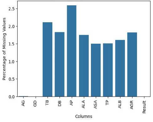
Fig. 2. Missing values (%) in each column

The values of all attributes in the dataset were normalized to a range between 0 and 1 using the min-max scaling technique, as described in Eq. (1) where x represents the attribute value, while x min and x max correspond to the minimum and maximum values of x, respectively.

x - x_min x scaled =

x max - x min

Table 5. Feature importance

Method	Algorithm	AG	GD	TB	DB	AP	ALA	ASA	TP	ALB	AGR
Bagging	RF	0.003	0.0005	0.113	0.079	0.165	0.160	0.153	0.113	0.111	0.099
	ETC	0.003	0.0016	0.120	0.104	0.141	0.144	0.128	0.113	0.118	0.123
Boosting	AdaBoost	0.005	0	0.058	0.033	0.317	0.160	0.205	0.074	0.080	0.064
	GradientBoost	0.000072	0.000010	0.146	0.069	0.200	0.174	0.145	0.068	0.098	0.096
	XGBoost	0.001	0.005	0.1634	0.1639	0.1187	0.1180	0.100	0.097	0.105	0.124
	CatBoost	0.023	0.001	10.635	8.291	15.127	15.966	14.947	10.069	11.993	12.943
	LightGBM	5459	122	4197	1934	9378	5398	7271	5982	5224	3605

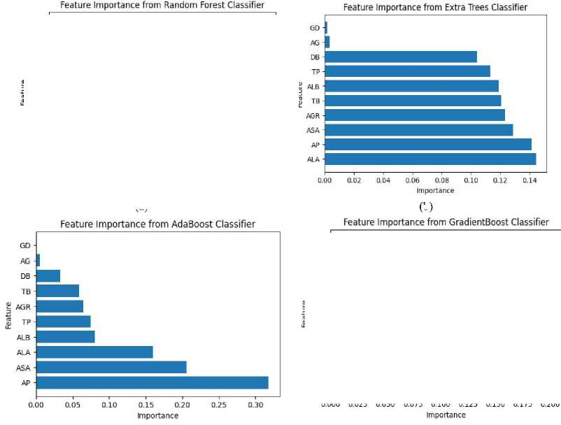
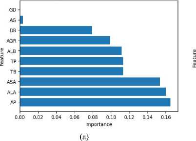
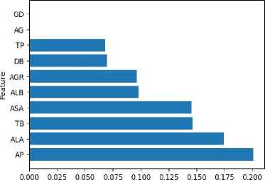
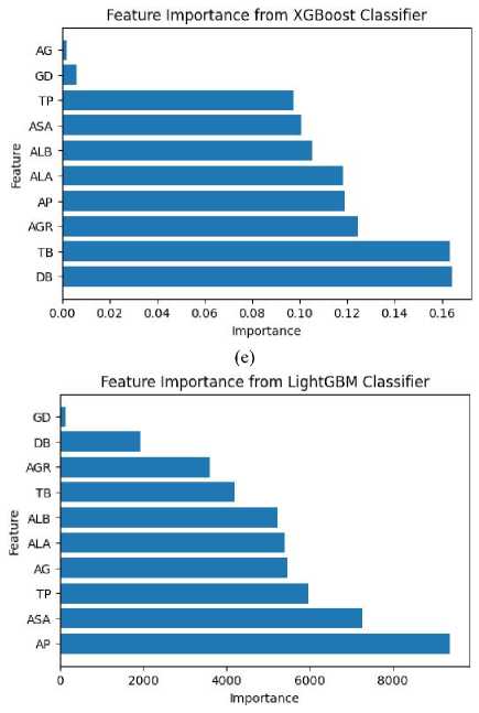
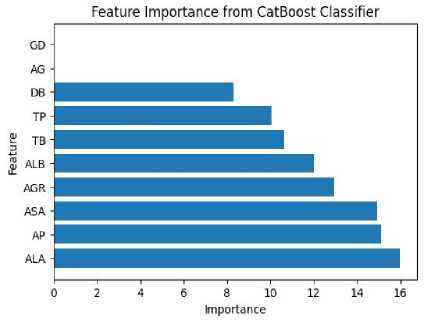
We have employed the feature importance score as a metric that plays a crucial role in predicting liver disease. Table 5 presents the contributions of each predictive attribute to liver disease prediction across different algorithms. For both bagging and boosting classifiers, the results indicate that attributes such as AP, ASA, and ALA are the most influential factors in prediction, consistently showing high significance scores.

Additionally, the table reveals that the attribute Gender (GD) was found to have a contribution of zero for AdaBoost and less significant than Age (AG) across all other algorithms. This finding suggests that every attribute provided at least some predictive value, regardless of the model used. As a result, only the GD attribute was eliminated during the analysis. Figure 3 provides a graphical representation of the significance of each attribute across different methods.

To detect outliers in the datasets, we also employed the Interquartile Range (IQR) method [28], which effectively highlights extreme values. This analysis revealed the presence of significant outliers, especially in the attributes DB, AP, and ALA. To handle these anomalies and minimize their influence on the data analysis, we applied the Z-score method (see Eq. 2), which standardizes data points and reduces the effect of extreme values. A visual representation of the outliers is provided in Figure 4, which illustrates the boxplots of these attributes, clearly highlighting the identified outliers and their distribution. After removing outliers (threshold value=3) from the dataset, the total number of data was reduced to 28,133 (Liver Patients: 19,410, Not Liver Patients: 8,723).

x_i -µ

Z - Score_i = σ

Where x i = each data point in the dataset, µ = mean of the dataset and σ = Standard deviation (see Eq. 3).

N

( x i -µ)²

(d)

(c)

=k

(b)

(g)

(f)

Fig. 3. Graphical representation of feature score of: (a-b) bagging and (c-g) boosting methods

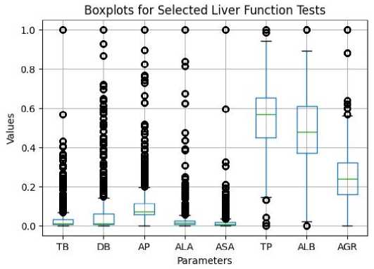
Fig. 4. Box plot representation of different attributes

• 4.    Experimental Setup, Results and Discussion

Table 6 shows the experimental setup and configuration details of liver disease prediction to conduct our work.

Table 6. Hardware and software tools to carry out the experiment

Hardware/Software	Specification
Processor	AMD Ryzen 7 5800U with Radeon Graphics @1.90 GHz
RAM	16.0 GB
Hard Disk	1 TB
Operating System	Windows 11
Programming Language	Python
Platform	Colab Notebooks

In this paper, we have conducted several analyses to evaluate different ensemble models for liver disease prediction. We have assessed the performance of each classifier using several key metrics, calculated from the confusion matrix presented in Table 7. These metrics include recall/sensitivity/true positive rate (TPR), specificity/true negative rate (TNR), precision, F1-score, miss rate/false negative rate (FNR), false positive rate (FPR), false discovery rate (FDR), overall accuracy/accuracy and Matthews Correlation Coefficient (MCC) which have summarized in Table 8. The confusion matrix provides a detailed breakdown of true positive (TP), true negative (TN), false positive (FP), and false negative (FN) predictions, enabling a comprehensive assessment of the model's effectiveness in classifying liver disease cases. We split our dataset as training (70%: 19,693) and testing (30%: 8,440).

Table 7. Confusion matrix

Actual class	Predicted class
	Positive	Negative
Positive	TP	FN
Negative	FP	TN

We have also used Receiver Operating Characteristics (ROC) curve (shows the graphical representation of true positive rate and false positive rate) as a performance metric to evaluate our work.

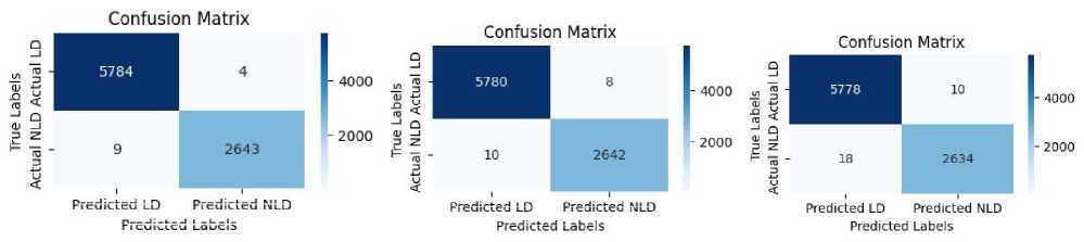
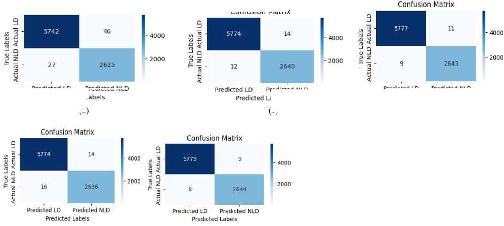
The confusion matrices for all classifiers are presented in Figure 5, while Table 9 summarizes the performance metrics for each classifier, derived from their respective confusion matrices. Figure 6 provides a graphical comparison of recall, precision, F1-score, and accuracy, highlighting the strengths and weaknesses of each method. Among boosting methods, LightGBM achieved the highest testing accuracy of 99.80%, demonstrating its exceptional predictive power whereas the lowest accuracy score was achieved by AdaBoost classifier. GradientBoost and CatBoost obtained almost the same accuracy of 99.69% and 99.64% respectively. On the other hand, RF obtained the highest classification rate (99.85%) as a bagging method. Experimental results indicate that the bagging approach (RF: 99.85%) slightly outperformed boosting method (LightGBM: 99.80%) in predicting liver disease.

Table 8. Performance metrics

Evaluation Metrics	Formula
Recall	TP TP + FN
Specificity	TN TN + FN
FPR	FP FP + TN
FNR	FN FN + TP
Precision	TP TP + FP
F1-score	Precision * Recall 2* Precision + Recall
Accuracy	TP + TN TP + TN + FP + FN
FDR	FP FP + TP
MCC	TP * TN - FP * FN sqrt ( ( TP + FP )*( TP + FN * ( TN + FP )*( TN + FN )

Table 9. Performance metrics of different classifiers

Method	Algorithm	Recall	Specificity	Precision	F1-score	Accur acy	FPR	FNR	FDR	MCC	TP	FP	TN	FN
Bagging	RF	99.84	99.85	99.93	99.89	99.85	0.15	0.16	0.07	99.64	5784	4	2643	9
	ETC	99.83	99.70	99.86	99.84	99.79	0.30	0.17	0.14	99.51	5780	8	2642	10
	Bagging DT	99.69	99.62	99.83	99.76	99.67	0.38	0.31	0.17	99.23	5778	10	2634	18
Boosting	AdaBoost	99.53	98.28	99.21	99.37	99.14	1.72	0.47	0.79	98	5742	46	2625	27
	GradientBoost	99.79	99.47	99.76	99.78	99.69	0.53	0.21	0.24	99.29	5774	14	2640	12
	XGBoost	99.84	99.59	99.81	99.83	99.76	0.41	0.16	0.19	99.45	5777	11	2643	9
	CatBoost	99.72	99.47	99.76	99.74	99.64	0.53	0.28	0.24	99.18	5774	14	2636	16
	LightGBM	99.86	99.66	99.84	99.85	99.80	0.34	0.14	0.16	99.53	5779	9	2644	8

Predirtsd I D

Predicted Nl П

Predicted LC

Predicted NLD

Predicted Labe s

Predicted Labe s

Predicted LD

Predicted NLD

(b)

(a)

(c)

Confusion Matrix

Confusion Matrix

Predicted I D Predicted NLD

Predicted LD Predicted NLD

Predicted

Predicted I D

Predicted Nl D

Predicted LC

Predicted NLD

(f)

(h)

(g)

Predicted LD Predicted NLD

Predicted Labels

Fig. 5. Confusion matrix of Bagging: (a) RF, (b) Extra Trees, (c) Bagging DT and boosting: (d) AdaBoost, (e) GradientBoost, (f) XGBoost, (g) CatBoost, (h) LightGBM algorithms

(d)

(e)

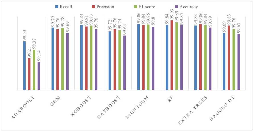
Fig. 6. Comparison of recall, precision, F1-score, and accuracy score

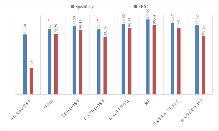
Fig. 7. Comparison of the algorithms based on positive performance metrics

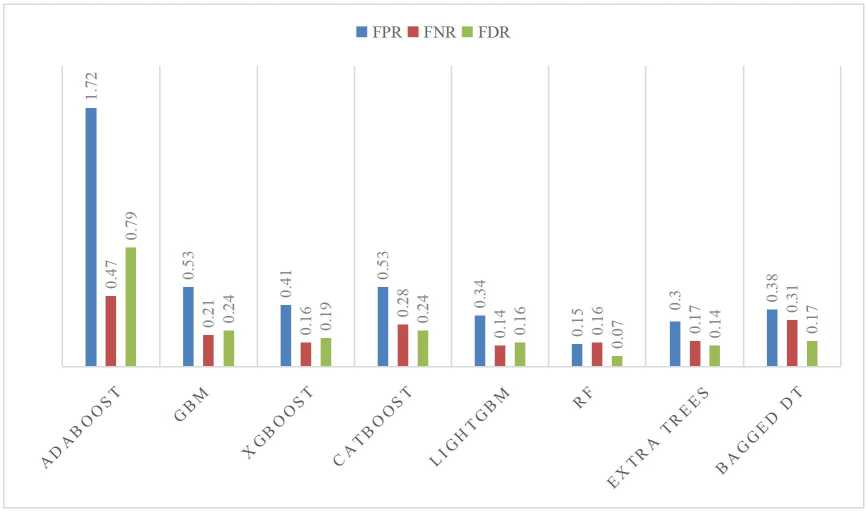
Fig. 8. Comparison of the algorithms based on negative performance metrics

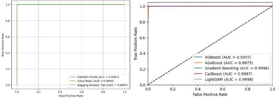
Figures 7 and 8 offer a more detailed comparison of the classifiers, focusing on both positive metrics (specificity, MCC) and negative metrics (TNR, FNR, FDR). Across all these measures, RF and LightGBM consistently outperformed other algorithms as bagging and boosting methods. To evaluate how well the algorithms can differentiate between TPR and FPR, we compared their performance using the AUC-ROC. The results of this comparison are illustrated in Figure 9, providing a clear visual representation of each algorithm's classification effectiveness.

(b)

(a)

Fig. 9. ROC Curve of: (a) bagging and (b) boosting methods

To better evaluate the performance of the proposed framework, we compared our results with several related studies using various evaluation metrics. As shown in Table 10, the proposed methodology achieved competitive performance compared with previous liver disease prediction studies conducted on both the ILPD and LDPD datasets. While earlier studies reported accuracies of up to 95.8% on the ILPD dataset and 98.80% on the LDPD dataset, our approach achieved an accuracy of 99.85% using Random Forest and a recall of 99.86% using LightGBM on the LDPD dataset.

Table 10. Comparison of our method with other published works on liver disease prediction

Paper	Algorithm Considered	Dataset Used	Recall	Specificity	Precision	F1-score	Highest Accuracy
[10]	GB, AdaBoost, LogitBoost, SGBoost, XGBoost, LightGBM, and CatBoost.	ILPD and LDPD	ILPD 100: GB LDPD 99.58: XGBoost	ILPD 100: GB LDPD 97.74: GB	ILPD 93.85 GB LDPD 99.08: GB	ILPD 97.69: GB LDPD 99.15: GB	ILPD 98.29: GB LDPD 98.80: GB
[8]	Logistic Regression, RF, XGBoost, SVM, AdaBoost, K-NN, and DT	ILPD	98.90: SVM	-	87: RF	90.16: RF	83.76: RF
[9]	TPE with DT, RF, ETC, LightGBM and AdaBoost	ILPD	96.3: ETC	-	95.5: ETC	95.8: ETC	95.8: ETC
[4]	XGB, LGBM, GB, BDT, RF, ET, Logistic Regression, DT and SVM	LDPD	99.74: XGB	97.74: GB	99.08: GB	99.15: GB	98.80: GB
[14]	LR, RF, KNN, SVM, MLP and ensemble	ILPD	92.97: SVM	-	93.36: KNN	91.83: KNN	93: KNN
Our	RF, ETC, Bagged DT AdaBoost, GradientBoost, XGBoost, CatBoost and LIghtGBM	LDPD	99.86: LightGBM	99.85: RF	99.93: RF	99.89: RF	99.85: RF

• 5.    Conclusion

In our research, we focused on the early prediction of liver disease based on ensemble learning and wanted to find the best model that could significantly advance the field of liver disease research. We investigated the performance of boosting and bagging as ensemble learning techniques. The boosting approach comprised five algorithms—AdaBoost, GradientBoost, XGBoost, CatBoost, and LightGBM—while the bagging approach included RF, Extra Trees, and Bagged DT. From experimental results, bagging algorithms particularly RF achieved the highest performance compared boosting algorithms with an accuracy, specificity, precision and F1-score of 99.85%, 99.85%, 99.93% and 99.89% respectively. However, LightGBM attained the highest level of recall (99.86%) among all the bagging and boosting algorithms. Additionally, Extra Trees and XGBoost also demonstrated satisfactory performance. In future work, we will incorporate advanced methods for handling imbalanced data and missing values and explore more extensive hyperparameter optimization using techniques such as Grid Search, Random Search, and Bayesian Optimization. Future studies will also investigate the integration of deep learning and explainable artificial intelligence approaches alongside k-fold crossvalidation and statistical significance testing to improve model performance, robustness, and interpretability.

All the Declarations and StatementsAuthor Contributions Statement

A. S. M. Shafi – Methodology, Formal analysis, Software, Writing-Original draft, Writing review and editing.

Conflict of Interest Statement

The author declares no conflicts of interest.

Funding Declaration

The authors declare that no external funding was received for this study.

Data Availability Statement

This study analyzed publicly available datasets. The results obtained and datasets can be found here: “”, accessed on “Jan 23, 2025”.

Ethical Declarations

Ethical approval was not required for this study as it did not involve human participants or animal experiments.

Acknowledgments

N/A

Declaration of Generative AI in Scholarly Writing

The author(s) declare that no generative artificial intelligence tools were used in the preparation of this manuscript.

Abbreviations

The following abbreviations are used in this manuscript:

Liver Diseases -LD

Random Forest-RF

Extra Trees Classifier-ETC

Bagged Decision Tree-Bagged DT

Adaptive Boosting-AdaBoost

Gradient Boosting-GradientBoost

Xtreme Gradient Boosting-XGBoost

Categorial Boosting-CatBoost

Light Gradient Boosting Machine-LightGBM

Machine Learning-ML

Indian Liver Patient Dataset-ILPD

Tree-Structured Parzen Estimator -TPE

Gradient Boosting-GB

Synthetic Minority Over-sampling Technique-SMOTE of K-Nearest Neighbor-KNN

Principle Component Analysis-PCA

Linear Discriminant Analysis-LDA

Factor Analysis-FA

Support Vector Machine-SVM

Multilayer Perceptron-MLP

Thoracic Surgery-TSD

Pima Indian Diabetes-PID

Chaotic Multi-Verse Optimization-CMVO neighbor-weighted KNN-NWKNN

Tomek Link and Redundancy-based Under-Sampling-TR-RUS

Gradient-based One-side Sampling-GOSS

Exclusive Feature Bundling-EFB

Interquartile Range-IQR

True Positive Rate-TPR

True Negative Rate-TNR

False Negative Rate-FNR

False Positive Rate-FPR

False Discovery Rate-FDR

Matthews Correlation Coefficient-MCC

True Positive-TP

True Negative-TN

False Positive-FP

False Negative-FN

A PPENDIX A\B\C…, with appendix tile

This study does not include any appendices.