Shelf Space Optimization in Retail: A Study Using Linear Programming, Genetic Algorithm, and Proximal Policy Optimization

Efficient management of retail shelf space plays a crucial role in maximizing profitability, enhancing inventory turnover, and improving customer satisfaction. In the dynamic and competitive landscape of modern retail, effective product placement and strategic space allocation significantly influence consumer purchasing behavior and operational efficiency. With increasing product variety, constrained shelf capacity, and fluctuating customer demand, traditional shelf management methods fall short in responsiveness and in decision making.

The current work proposes integrated shelf space optimization framework that leverages advanced data analytics and optimization techniques to address these challenges. The system combines predictive modeling, sales analytics, and optimization algorithms to offer data-driven support for strategic shelf planning. A robust and interactive dashboard is developed to visualize critical sales metrics, track product performance, and filter data by seasonal and categorical parameters. Additionally, a forecasting module, powered by Prophet, anticipates product demand to guide timely shelf adjustments and inventory decisions. A hybrid LP–GA–PPO framework methods are employed to enhance shelf allocation: Linear Programming (LP) for mathematically precise solutions, Genetic Algorithm (GA) for navigating complex, high-dimensional solution spaces, and Proximal Policy Optimization (PPO), a reinforcement learning approach enabling dynamic and adaptive decision-making. The system is designed to be scalable across various retail formats and customizable to different store sizes and product categories. The integration of predictive analytics, intelligent optimization, and visual decision aids addresses key industry pain points such as inefficient space utilization, inaccurate demand forecasts, and lack of actionable insights. By unifying these components, the proposed model empowers retailers with a strategic and adaptable solution for real-time, high-impact shelf space management. The proposed work presents a comparative evaluation between deterministic, evolutionary, and reinforcement learning approaches for retail shelf optimization under realistic constraints compared to the existing work.

2.    Related Works

Shelf space optimization plays a critical role in retail operations by directly influencing product visibility, inventory turnover, and overall sales performance. As the retail industry embraces data-driven decision-making and AI-based technologies, researchers have explored a variety of models and algorithms to address the challenges of shelf space allocation, inventory control, and demand forecasting. This section presents a comprehensive review of relevant research contributions, categorizing them based on their alignment with our project’s modules: forecasting, optimization, dashboard integration, and system scalability. Supply Chain 4.0 influences digital technologies such as AI, IoT and big data to create real-time, demand-driven operations, by ensuring the right products are placed in the right quantities at the right time [1]. The proposed work advances the integration of LP, GA and PPO. This integration reduces stockouts, minimizes excess inventory, and enhances customer satisfaction. In a systematic literature review [2], the authors highlight a wide range of approaches to the Shelf Space Allocation Problem (SSAP), pointing to the need for intelligent, adaptable methods in modern retail environments. Riazi [3] proposed an inventory control strategy for profitable perishable goods, which aligns closely with our forecasting objective using seasonal data. Author [4] introduced a biobjective optimization model integrating assortment, promotion, shelf allocation, and inventory replenishment, providing direct inspiration for the integrated structure of our proposed framework. Similarly, Ostermeier [5] provided a full-store allocation model that serves as a structural reference for our system wide optimization logic. Gencosman and Begen [6] explored exact and decomposition-based strategies for optimizing shelf space. Their use of LP reinforces our implementation of Linear Programming to guarantee optimal outcomes under defined constraints. Czerniachowska [7] proposed a Genetic Algorithm for virtual segment shelf space allocation, which inspired our use of GA to tackle highdimensional and dynamic layout scenarios. Murray [8] tackled the joint optimization of pricing, shelf display, and product orientation, underscoring the importance of multi-parameter tuning—an aspect we address through Proximal Policy Optimization (PPO). Sajadi and Ahmadi [9] ex-tended this idea by integrating assortment planning, shelf space allocation, and replenishment in a real application, which validated our multi-layered optimization structure. Czerniachowska and Hernes [10] focused on heuristic support systems, incorporating visual shelf factors like capping and facings. These findings influenced our dashboard visualization logic, especially in the interactive planogram module. The authors proposed re-allocation techniques to reduce out-of-stock scenarios, emphasizing the importance of dynamic forecasting goal served by our Prophet-based forecasting pipeline [11]. Flamand [12] showed that grouped product displays could increase impulse purchases, which we translated into our category-based allocation filters. Higuchi and Takeyasu [13] presented an expanded GA based shelf planning model, further supporting the adaptability of our GA component. Rautaray [14] suggested using big data for shelf planning, which supports our use of scalable frameworks and interactive tools like Streamlit and Plotly. Duan [15] discussed the opportunity cost of store brand placements, suggesting potential pricing integration in future versions of our system. Gajjar and Adil [16] linked shelf space allocation with replenishment strategies, which rein-forces our data-driven link between forecasting and allocation. Geismar [17] introduced two-dimensional space optimization to maximize revenue, aligning with our model’s ability to evaluate across multiple axes (profit, space, category). Digital supply chain practices in manufacturing boost company performance by improving demand forecasting, inventory visibility, and decision making, contributes to effective shelf space optimization in retail sectors by khan [18]. A model is developed to maximize a retailer’s profit when demand is stochastic by selecting the number of facings and their shelf position by Hubne [19]. Though recent studies have integrated optimization models, there are some research gaps remaining like focus on using only one optimization method, limited attention has been given to translating outcomes into practical decision support tools that retail planners can interact with and finally PPO remains underexplored compared to traditional techniques. The proposed work addresses these gaps with the development of dashboard-based framework to visualize the allocation strategies and enabling quantitative performance evaluation.

Fig. 1. Detailed Flow Chart of Data Processing and Module Execution

Figure 1 shows the flowchart of the work. Following are the steps to understand the flow of implementation:

Step 1: Data Ingestion: The user initiates the process by uploading a CSV file containing raw sales and product metadata. The upload_and_preview_data() helper function reads the file, automatically detects common date formats, and coerces invalid dates to NaT (which are later dropped). Simultaneously, a new column Shelf_Area is computed as Width_cm x Height_cm to capture the physical space requirement for each product. If the upload fails (wrong file type or unreadable content), the flow charts back to an error handler that displays an explanatory message and prompts the user to retry.

Step 2: Preprocessing & Filtering: Once ingestion succeeds, the raw DataFrame enters a validation stage: Rows with missing critical fields (Product_Name, Expiry_Date) are dropped. Outliers in numeric fields may be flagged for review or automatically clipped to reasonable bounds. The user is then presented with three filter controls:

• •    Season Selector: Picks one or more seasons (e.g., “Summer”, “All Season”).

• •    Category Filter: Narrows to specific product categories (e.g., “Beverages”, “Snacks”).

• •    Profit Range: Defines a lower and upper bound on per-unit profit.

“Apply Filters” action produces a Filtered Data subset, which drives all downstream modules in parallel.

Step 3: Module Execution (Branching Logic):

• i.    Dashboard Module (dashboard.py): Computes key performance metrics (total sales, average profit, product turnover). Generates visualizations: sales by category, size-based profit breakdown, expiry vs. sales scatter. Renders interactive tables for Top N products and time-series drilldowns.

• ii.    Forecasting Module (forecast.py): Accepts user-specified Forecast Horizon and Volatility Multiplier. Fits a Prophet model to historical data and decomposes time series into trend, seasonality, and residuals. Runs a Monte Carlo inventory simulation for the projected horizon, outputting expected stockouts and average inventory levels. Produces two chart types: “Forecast vs. History” and “Sample Inventory Trajectories”.

• iii.    Optimization Module (optimization.py): Presents algorithm choices: Linear Programming, Genetic Algorithm, or PPO Reinforcement Learning. Translates filtered data and forecasted demand into optimization constraints (shelf area limits, category weights). Solves for an optimal planogram layout, balancing predicted sales against shelf real estate. Create a downloadable planogram mapping each product to fixed shelf coordinates.

Step 4: Output generation: As each module completes, its results are sent back to the Streamlit UI: Charts and tables appear in dedicated tabs. Simulation statistics and trade-off curves are displayed with explanatory tooltips. A unified “Download” button lets the user export: The processed CSV (with all computed fields and filtered rows). The finalized planogram in CSV or image format. If any module encounters an error (e.g., model convergence failure, infeasible optimization), a descriptive alert guides the user to adjust filters or parameters.

The optimization problem aims to allocate available shelf capacity, where equation 1 shows objective function to maximize profit and satisfies the space and demand constraints:

max Z = X ?=i P i x_t

Where: P i represents the profit contribution of product i,x i represents allocated shelf space. The equation 2 and 3 gives shelf capacity constraint and demand constraints:

n

S i X t t=1

Where: s i is shelf size required by product (, S is total available shelf capacity.

X i <  d t                                                        (3)

• 3.1.    Framework diagram

Figure 2 and 3 presents the overall framework, which is organized into four logical layers:

• i.    Ingestion Layer: A single CSV upload endpoint reads raw sales and product data, standardizes formats, and computes derived fields (e.g. Shelf Area).

• ii.    Shared Data Cache: The cleaned DataFrame is held in memory once, ensuring that all downstream modules operate on an identical, preprocessed dataset without redundant I/O.

• iii.    Module Layer:

• a.    Dashboard: Enables interactive analytics with charts, tables, and key performance indicators (KPIs).

• b.    Forecast: Projects demand using Prophet model and synthetic simulation techniques.

• c.    Optimize: Generates planograms using optimization algorithms like Linear Programming (LP), Genetic Algorithm (GA), and Proximal Policy Optimization (PPO).

• iv.    Output Layer: A unified “Download” control exposes module-specific exports filtered CSVs, charts, simulation metrics, or planogram files directly to the user.

4.    Implementation

• 4.1.    System Architecture Overview

This section emphasizes how dynamic shelf space allocation problems have been addressed through modular design, reactive user interfaces, and advanced optimization techniques. End-to-end workflow is examined from data ingestion and interactive visualization to forecast and multi-method allocation engines, highlighting performance, scalability, and user experience considerations.

At startup, app.py establishes the application shell, configures global CSS, and initializes Streamlit’s session state to manage page navigation. A centralized router handles three core pages: Dashboard, Forecast, and Optimization ensuring a seamless multipage experience without external dependencies. All shared utilities (data loaders, parsers, filters) reside in utils/helpers.py, promoting DRY principles and enabling consistent behavior across modules. Key architectural patterns include:

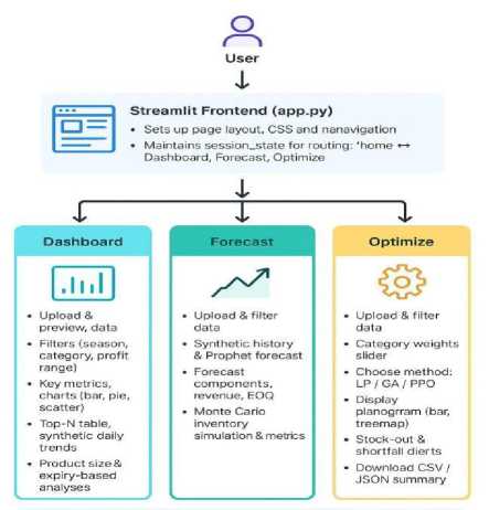
Fig. 2. Framework diagram of the Shelf Space Optimization System

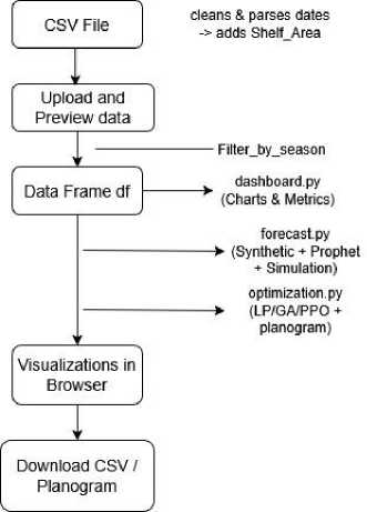
Fig. 3. Data Flow Diagram of Modules and Data Stores

• •    Reactive UI Model: Leveraging Streamlit’s rerun-on- widget-change semantics, each user interaction triggers an efficient diff-based re-execution, preserving application state and minimizing latency.

• •    Session State Management : Distinct session keys (e.g., dashboard_season, forecast_season, opt_season) isolate user inputs per module, preventing cross-page collisions and enabling true multi-tab support.

• •    Modular Utilities: upload_and_preview_data() and filter_by_season() encapsulate data validation, type coercion (dates, numeric fields), and basic feature engineering (e.g., computing Shelf_Area). This centralization simplifies maintenance and ensures consistency.

• 4.2.    Dashboard Module

• i.    Data Ingestion and Preprocessing: Users upload a CSV via Streamlit’s file_uploader. Internally, the helper functions:

• •    Reads data with Pandas, handling common encodings and CSV quirks.

• •    Parses Expiry_Date across multiple date formats, coercing invalid entries to NaT and filtering them out.

• •    Computes derived features such as Shelf_Area and validate numeric columns, issuing warnings for missing critical fields.

This early validation loop guarantees that downstream filters and charts operate on a clean, predictable DataFrame.

• ii.    Dynamic Filtering Pipeline: Three sequential filters refine the dataset:

• •    Season Selection : A selectbox triggers filter_by_season(), which uses case-insensitive string matching to accommodate user input variations.

• •    Category Multi-Select : Available categories are derived from the seasonally filtered set, ensuring relevancy. The multiselect component allows multi-category comparison and automatically synchronizes with season changes.

• •    Profit Range Slider : Using the filtered DataFrame’s min/max values, the slider bounds update dynamically, preventing user selection of out-of-range values.

• iii.    Visualization and Metrics:

Key Performance Indicators: A three-column layout leverages st.columns to display:

• •    Total Sales (30d): Sum of Sales_Last_30_Days via vectorized operations.

• •    Avg Profit/Unit: Computed as the mean of Profit_Per_Unit to two decimal places.

• •    Total Profit (30d): Product sum of sales and profit columns.

• iv.    Interactive Charts: Plotly powers three main visuals:

Sales by Category, Sales vs. Profit Scatter and Top N Products Table.

• v.    Synthetic Daily Trends: Triggered by a checkbox, synthetic time series generation

• 4.3.    Supply Forecast Module

The Forecast module extends the Dashboard by projecting demand and guiding inventory decisions:

• i.    Synthetic History and Model Training:

Synthetic History Generation : Users can adjust volatility via a slider. We generate 30-day demand traces using NumPy’s random normal distribution, anchoring on average daily sales to illustrate stochastic demand scenarios.

ProphetIntegration :     Instantiating Prophet(daily_seasonality=True),

Indian holidays are added (model.add_country_holidays (country_nam e=’IN’)) to capture cultural seasonality. The model is fitted on the synthetic series inside a Streamlit spinner, ensuring responsive feedback during training.

• ii.    Forecast Visualization and Components:

• •    Forecast vs. History Plot: Overlaid scatter (history) and line (forecast) traces highlight model performance.

• •    Component    Decomposition: Using model.plot_components(), users explore trends, weekly seasonality,

• 4.4.    Revenue Forecast

and holiday impact, illustrating how each factor contributes to predicted demand.

Demand Planning Metrics: Safety stock and reorder points are computed using the standard formula below:

SS = zx a^LT and ROP = px LT + SS

2DS where z is the service-level z -score and LT is lead time. EOQ is calculated as \-- demonstrating classical inventory management principles. Interactive Monte Carlo Inventory Simulation: Within an expander, users configure initial inventory and run count. The simulate_inventory() routine executes multiple demand vs. inventory simulations, returning:

• •    Avg. Stockouts per Sim: Mean count of days with unmet demand.

• •    Avg. Ending Inventory: Typical on-hand stock at horizon’s end.

• •    Histograms and Trajectories: Visual distributions and sample path plots, aiding risk assessment and safety stock calibration.

• 4.5.    Shelf Space Optimization Module

Addressing the dynamic shelf space allocation problem, the Optimization module computes profit-maximizing placements under capacity constraints:

• i.    Priority Weighting and Capacity: Users assign weights to each category (defaulted via normalized seasonal sales) to capture strategic priorities. The total_space slider sets the hard shelf unit limit, instantly re-triggering the allocation algorithms.

• ii.    Optimization Engines:

• a.    Linear Programming (LP): Formulated as:

  s. t

  
  
  
  

  max£ j W 1 P1X 1

  
  

  x_t< C,x_t > 0,x_t E Z

  
  
  
  

where W [ is the category weight, p_t is unit profit, and C is capacity. Solved via optimize_lp().

• b.    Genetic Algorithm (GA): A population of allocation vectors evolves over generations using crossover and mutation operators, balancing exploration and exploitation. Progress logs and convergence metrics are displayed to the user.

• c.    PPO (Reinforcement Learning): An RL agent trained using Proximal Policy Optimization treats allocation as a sequential decision task. The optimize_ppo_speedup() function runs multiple parallel environments for sample efficiency, and training progress is conveyed via a spinner and final policy evaluation metrics.

Result Visualization and Alerts:   Regardless of the chosen method, results are fed into display_planogram_interactive (), producing:

• •    Category-Level Bars: Summarize total units per category.

• •    Product-Level Bars: Detail individual allocations, color- coded by category.

• •    Treemap View: Reveals proportional usage, providing both macro and micro perspectives.

• 4.6.    Performance and Caching Strategies

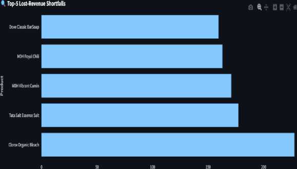
Additionally, a post-allocation alert system: Computes Ideal Allocation vs. actual allocations to identify shortfall units. Aggregates Lost Revenue per product, sorting by highest impact. Presents interactive tables and charts (bar and pie) to highlight top at-risk products and category-level revenue exposure.

To maintain responsiveness under heavy computation, we employ several strategies:

• i.    Streamlit Caching: Critical functions like synthetic history generator, GA optimizer is decorated with @st. cache_data to prevent redundant recomputation when inputs remain unchanged.

• ii.    Lazy Loading: Large DataFrames and heavy computations are deferred until explicit user actions, minimizing initial load times and memory usage.

• iii.    Asynchronous Feedback: Spinners (via with st.spinner()) and progress bars inform users of long-running tasks, keeping the UI responsive and preventing lockups.

5.    Results 5.1.    Experimental Setup

The implementation weaves together dynamic data ingestion, interactive visualization, probabilistic forecasting, and multi-method optimization into a coherent, user- centric application. By decoupling modules, applying rigorous caching, and providing real-time responsiveness, a powerful tool for dynamic shelf space allocation is delivered that scales from small boutiques to enterprise operations.

This section presents the experimental results and comparative evaluation of different shelf space optimization techniques PPO, GA and LP under different seasonal constraints.

• •    Platform: Python 3.10 with Streamlit interface.

• •    Libraries: NumPy, Pandas, Plotly, Prophet, DEAP, SciPy, and PyTorch.

• •    Frontend: Interactive dashboard allowing seasonal input, category weight adjustment, and visual analytics.

• •    Shelf Units Constraint: Fixed at 5000 units for all experiments.

• i.    Seasonal Filtering and Performance Insights: Figure 4 illustrates how users can upload the retail dataset and select a specific season for analysis. Products can be filtered by category and a profit-per-unit slider to focus on target margins. The dashboard displays key performance indicators such as total sales, average profit per unit, and overall profit, supporting seasonal and category-based decision making.

• ii.    Sales Visualization by Category: Figure 5 presents a pie chart depicting the distribution of unit sales across categories. This visualization allows for a quick understanding of which categories dominate sales and offers a high- level comparison useful for inventory and marketing decisions.

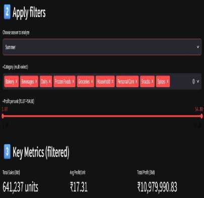
Fig. 4. Seasonal Filtering and Performance Insights (Summer, 5000 Rows)

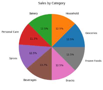
Fig. 5. Pie Chart Showing Proportion of Units Sold by Product Category (Filtered by Season and Category)

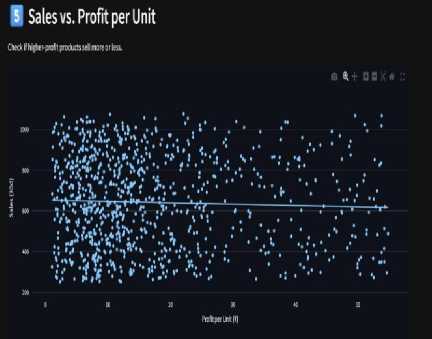
Fig. 6. Scatter Plot – Profit per Unit vs. Sales (Last 30 Days)

• iii.    Sales vs. Profit per Unit Scatter Plot Analysis: Figure 6 shows a scatter plot used to analyze the relationship between profit per unit and sales volume over the last 30 days. Each point represents a product, and tooltips reveal additional details on hover. A trendline assists in identifying pricing strategies and performance clusters.

Table 1. Top N Products Ranked by Sales (Last 30 Days)

Product_Name	Category	Sales_Last_30_Days	Profit_Per_Unit
MDH Urban Cumin	Spices	1076	22.07
Tropicana Vibrant Juice	Beverages	1073	10.3
Britannia Pure Cake	Bakery	1067	53.77
McCain Deluxe Nuggets	Frozen Foods	1067	49.53
Head & Shoulders Fresh Shampoo	Personal Care	1061	3
Lysol Savory Disinfectant	Household	1060	6.64
Ritz Classic Crackers	Snacks	1057	15.8
Green Giant Royal VegMix	Frozen Foods	1054	22.78
Ritz Royal Crackers	Snacks	1052	17.6
Tropicana Urban Juice	Beverages	1048	5.7

• iv.    Top N Products by Sales: Table 1 displays a ranked list of top-performing products based on sales in the past 30 days. A slider allows dynamic selection of N (e.g., Top 5, Top 1), enabling retailers to quickly spot high-volume items and optimize inventory and placement accordingly for N=18.

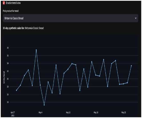
Fig. 8. Synthetic 30-Day Sales Trend for Selected Product

• v.    Synthetic Daily Sales Trend for Selected Product: Figure 8 illustrates a simulated 30-day sales trend for a chosen product, generated using average daily sales with random fluctuations. This aids in visualizing demand cycles even when real-time sales data is sparse or unavailable.

• 5.2.    Explanation of Supply Forecast section

• i.    Season and Product Selection with Key Metrics: The Forecast module lets users upload data, pick a season, and select a product from the filtered list. It then shows key metrics like total sales in the last 30 days and average daily sales, providing tailored forecasts based on season and product trends as shown in figure 9.

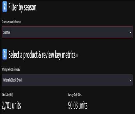
Fig. 9. Key Metrics of Britannia Classic Bread(Summer,5000rows)

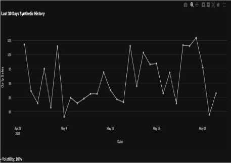
Fig. 10. Synthetic 30-day sales graph with realistic fluctuations showing recent trends

• ii.    Forecast settings: Configure the forecast parameters to simulate future sales. Two key settings are provided: forecast horizon, which determines the number of days to predict ahead (ranging from 7 to 60 days), and volatility, which adjusts the variability of the synthetic sales history. These inputs allow users to explore different forecasting scenarios and understand potential fluctuations in product demand.

• iii.    Generate synthetic 30-day history: Figure 10 generates a 30-day synthetic sales history by adding controlled noise to average daily sales, simulating realistic fluctuations. It helps visualize past sales variability, enhancing forecast accuracy.

• iv.    Fit Prophet and forecast for the next 15 days: The Prophet forecasting model is trained on the synthetic 30-day sales history to capture underlying trends and seasonality, including country-specific holidays. Using this model, a 15-day forecast is generated, predicting future sales and highlighting short-term demand patterns to assist in inventory planning.

• v.    Revenue Forecast: This section calculates and visualizes the forecasted revenue over the selected horizon by multiplying predicted sales with the product’s profit per unit. The cumulative revenue metric provides a quick overview of expected earnings, while the bar chart shows daily revenue trends, aiding financial planning and decision- making.

• 5.3.    Optimization Techniques

While three algorithms—LP, GA, and PPO are implemented, this section displays results from the PPO algorithm, focusing solely on maximizing overall profit.

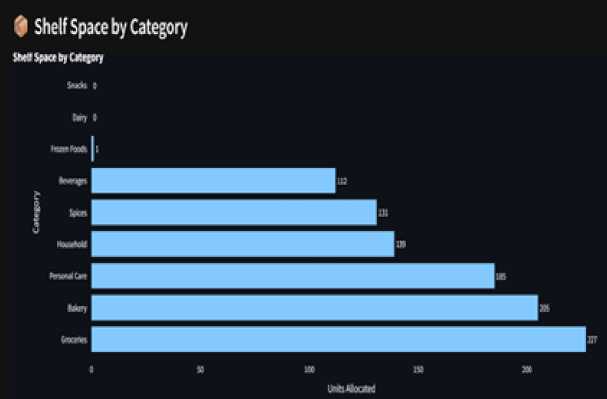
Fig. 11. Shelf space allocated to each category

• i.    Shelf Space by Category: Figure 11 visualizes the total shelf space allocated to each product category after optimization. The horizontal bar chart ranks categories by their allocated units, helping users quickly see which categories are prioritized in the shelf layout. This insight supports informed decisions on inventory distribution and space management aligned with business goals.

• ii.    Shelf Space by Product: Figure 12 presents a horizontal bar chart showing shelf space allocation for individual products, sorted by allocated units. Each bar is color-coded by category, with profit per unit available on hover. This view helps identify which products are prioritized on shelves, supporting detailed inventory and space management decisions.

9 Shelf Space by Product

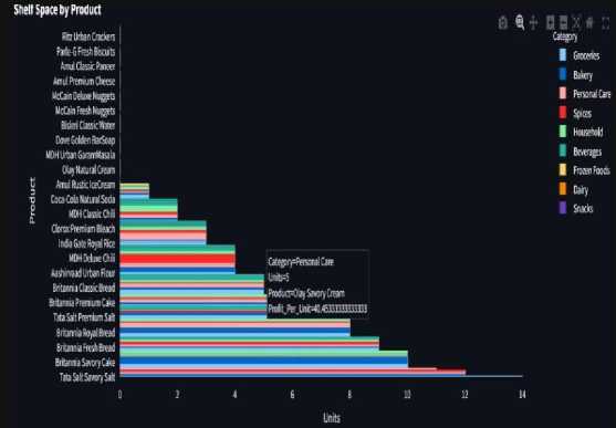
Fig. 12. Shelf space allocated to each product

• iii.    Proportional View (Treemap): Figure 13 visualizes shelf space allocation hierarchically by category and product. Categories are sized by total allocated units, with average category profit shown on hover. Individual products are nested within categories, sized by their allocated space and annotated with their profit per unit. This view offers an intuitive snapshot of how shelf space and profitability are distributed across the product range.

• iv.    Potential Stock-Out Alerts: Figure 14 highlights products at risk of stock-outs due to insufficient shelf allocation. If no risks are detected, it confirms all products are well stocked. Otherwise, it displays the number of at-risk products and estimated lost revenue, with an option to preview detailed data for top products based on potential revenue loss. Currently, the top 4 products by lost revenue are shown based on the user’s selection.

• v.    Top 5 Lost-Revenue Shortfalls: Figure 15 presents a horizontal bar chart of the top five products with the highest potential revenue loss due to under- allocation. It visually highlights which stock-outs could impact revenue the most, helping prioritize corrective actions.

• vi.    Category Share of Lost Revenue: The pie chart in Figure 16 shows how lost revenue from stock shortfalls is distributed across categories, based on the top 5 products with the highest shortfall impact. Users can adjust the number of products n to analyze, helping identify which categories contribute most to potential revenue loss and refine stocking strategies.

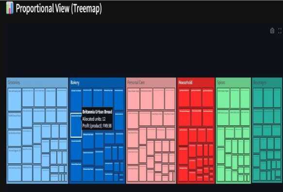
Fig. 13. Shelf Allocation Treemap — PPO Algorithm (Summer, 5000 Rows)

A Potential Stock-Out Alerts

Products at Risk

Total Lost Revenue

79,192.67

How many products to preview?

Showing top 4 products by lost revenue

Product.Name	Category	Sales_Last_3Q_Days Allocated.Space	ideal_Allocatlon	Shortfall-Units	Shortfall-Revenue
62 Clorox Organic Bleach	Household	5196	0	6	6                 227.698
153 Tata Salt Essence Salt	Groceries	7203	0		5                  177.24
119 МОП Vibrant Cumin	Spices	7179	0		6                  170.85
112 MDH Royal Chili	Spices	6324	0		6                 162.894

Fig. 14. Displaying number of products at risk, total lost revenue, top products at risk of stock-out.

Lost Revenue

Fig. 15. Top 5 Lost-Revenue Shortfall Products (PPO, Summer)

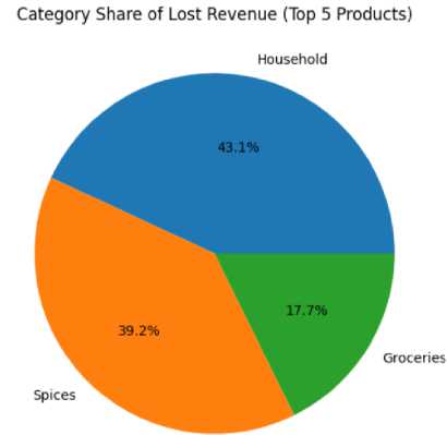
Fig. 16. Category Share of Lost Revenue Top 5 Products (PPO, Summer)

• 5.4.    Evaluation Metrics

• ○    Estimated Profit () : Total projected profit from allocated products.

• ○    Products at Risk: Number of products with demand exceeding supply (stock-out risk).

• ○    Lost Revenue (): Profit loss due to stock-outs.

As shown in Table 2, depending on the evaluation criterion, the relative performance of LP, GA, and PPO varies across seasonal scenario. PPO achieved the highest profit-oriented allocations during the Monsoon season, indicating its ability to adapt shelf-space decisions according to seasonal demand patterns. Furthermore, this profit improvement was accompanied by higher stock-out risk compared to GA. In contrast, GA exhibited more conservative allocation behavior and achieved lower or zero stock-outs during the winter season, resulting in improved inventory stability. LP produced the highest profit in certain summer while maintaining moderate risk levels. These results suggest that no single algorithm consistently dominates across all performance metrics; rather, the choice of optimization method depends on whether the retailer prioritizes profit maximization, inventory availability, or a balance between the two objectives.

Table 2. Optimization comparison across methods and seasons

Method	Season	Shelf units	Rows	Estimated Profit()	Product at Risk	Last Revenue()
PPO	Monsoon	5000	10000	144053.75	310	33277.00
GA	Monsoon	5000	10000	118486.67	1	26.13
LP	Monsoon	5000	10000	Infeasible	Infeasible	Infeasible
GA	Winter	5000	10000	113805.76	0	0.00
PPO	Winter	5000	10000	137700.12	305	31956.16
PPO	Summer	5000	5000	182006.13	152	35872.99
GA	Summer	5000	5000	145714.99	-	-
LP	Summer	5000	5000	208722.89	82	11154.96

Insights and Observations

• •    Proximal Policy Optimization achieves a good balance between profit maximization and stock- out risk minimization. Its reinforcement learning framework allows the model to adapt dynamically to varying data scales, seasonal demand patterns, and complex constraints. In high-volume datasets (e.g., 10,000 rows), PPO consistently outperforms heuristic methods in finding near-optimal allocations while minimizing critical product shortages.

• •    Linear Programming demonstrates the highest theoretical profitability under ideal, feasible constraint sets. However, it suffers significantly in scenarios with overlapping or conflicting constraints such as the Monsoon season case, where it becomes mathematically infeasible to allocate space while satisfying all defined conditions. This limits LP’s applicability in real-world, high-dimensional, and dynamic retail environments.

• •    Genetic Algorithm proves to be highly effective for moderate-sized datasets and seasonal variations. Its population-based search process, inspired by natural evolution, helps escape local optima and find diverse, valid solutions. GA is especially robust under uncertainty and shows minimal product stock-outs, making it a reliable choice when model interpretability and feasibility are prioritized over maximum theoretical profit.

6.    Conclusion

Dynamic shelf space allocation remains a critical challenge for modern retailers, driven by fluctuating demand, limited shelf area, and seasonal variation. Three distinct optimization approaches were implemented and evaluated such as PPO , which is a reinforcement learning method that dynamically learns the best allocation policy by maximizing cumulative reward based on forecasted demand and profit. Second one is GA, a robust, heuristic-based approach well suited for medium-scale retail datasets, balancing exploration and exploitation effectively. Last one is LP , a classical optimization strategy that offered high profits under feasible constraints but struggled with infeasibility in over constrained or highly variable data scenarios. The proposed work in the paper addressed key retail constraints including limited shelf capacity, product demand, and profitability objectives. Experimental evaluation demonstrated that LP provided efficient deterministic allocation under fixed constraints, while GA improved search flexibility for complex optimization scenarios. PPO further enabled adaptive decision-making by learning allocation strategies dynamically from the retail environment. Further, we can enhance using include real world scenarios, which include larger datasets, repeated trials to enable statistical validation.

The developed system supports practical retail planning through visualization and real-time allocation analysis, enabling better utilization of shelf space and improved profit-oriented decision-making. The comparative analysis highlights the strengths of combining classical and reinforcement approaches for modern retail applications. Future work may focus on incorporating real-time sales data, customer behaviour patterns, and additional operational constraints to further improve adaptive shelf allocation performance in large-scale retail settings.

All the Declarations and StatementsAuthor Contributions Statement

Anitha Palakshappa – Conceptualization and Supervision: Constructed the overall framework, and supervised project execution. Review and Editing, and Project Management. Reviewed and edited the manuscript, ensured clarity and coherence, and helped coordinate project milestones and deadlines.

Shruti J. R. – Writing – Drafted the initial manuscript, contributed to the literature survey.

Sowmya Kyatanahalli Nanjappa – Model Training, and Validation,

Ashwitha Anni – Documented the technical background of the study.

Aditya Gaonkar – Data Curation and Software Implementation: Handled data acquisition, dataset preprocessing, and implementing the research model.

Aditya Gaonkar – Performed in-depth analysis of experimental results, prepared performance charts, and ensured the statistical robustness of the evaluation.

All authors have read and agreed to the published version of the manuscript.

Conflict of Interest Statement

The authors declare no conflicts of interest.

Funding Declaration

The authors declared that there is no funding received for the work.

Data Availability Statement

This study analyzed publicly available datasets. Our application relies on a comprehensive product sales dataset comprising 10,005 records of consumer goods variants tailored for the Indian retail context. A synthetic retail dataset containing 10,005 product-variant records was generated to emulate the characteristics of Indian FMCG retail environments. Product names and categories were inspired by commonly available consumer goods, while seasonal attributes, sales volumes, and profit margins were generated within realistic ranges to facilitate comparative evaluation of shelf-space optimization algorithms.

The dataset will be made available on request.

Ethical Declarations

The authors should declare the following: There is no human subjects or animals used for the study.

Acknowledgments

The authors like to thank Ramaiah Institute of Technology for the support to conduct the research work. We sincerely thank the experts for their professional evaluation and valuable recommendations, which have contributed to improving the quality of the experiment and the reliability of its results.

Declaration of Generative AI in Scholarly Writing