TRAC: PCU-Weighted Traffic Control with Virtual Lanes for Unstructured Indian Traffic

The average travel time in major cities of India like New Delhi, Bengaluru, Kolkata, Mumbai and Chennai has risen significantly during peak hours. These metropolitan cities play a major role in our economy, experiencing rapid growth and significant urban transformations. The conventional traffic signal system operates based on a pre-set schedule stored in its memory without considering real-time traffic conditions [1]. Such inflexibility often leads to congestion, and the resulting bottlenecks have the potential to attract drivers to dangerous behaviors, such as speeding, thus increasing the potential for accidents. Contemporary traffic management systems usually have a difficult time coping with dense traffic flows, requiring manual intervention by traffic police. This type of operation is inherently difficult and inefficient and requires significant human input [2]. Although automatic traffic systems have been deployed, congestion is still a prevailing problem especially on roads with multiple intersections. Existing infrastructure is not well equipped to handle the explosive increase in the number of vehicles and the ever-increasing road network. Consequently, the deployment of an intelligent traffic control system is imperative for fine-tuning the traffic management system and easing the flow and congestion.

This work is open access and licensed under the Creative Commons CC BY 4.0 License.

These traffic problems have led to the use of inductive loops and infrared sensors in traffic management [3]. Nevertheless, they have some limitations, such as being localized for detection and being vulnerable to environmental factors. Further developments have suggested combining the Internet of Things (IoT) and Adaptive Neuro-Fuzzy Inference Systems (ANFIS) for intelligent traffic light control, and presenting potential improvements in traffic conditions by the traffic light control system in the future. [4] Moreover, vehicle to vehicle communication systems aim to improve signal management by exchanging real-time traffic data between vehicles and fixed nodes at intersections [5]. While promising, issues like the high cost of installation and intricacy of the system still remain. These innovations represent continued efforts to optimize traffic control systems to be as efficient and convenient as possible. Recently, image processing techniques have emerged as a viable solution for tackling traffic issues due to their simplicity of maintenance and smart capabilities. These techniques are commonly employed to detect vehicle edges and quantify traffic volume on roads [6]. This design project uses image processing techniques to develop a smart traffic light system for more effective traffic management. Prior intelligent algorithms have used techniques such as weighted average to calculate green signal time [7]. This approach has various disadvantages such as wastage of time when a lane is empty and starvation when there is consistent traffic from a particular lane. In order to overcome these disadvantages and improve the efficiency of the algorithm, a new algorithm is developed which will assist in clearing congested traffic and shortening commute time.

The proposed Traffic Routing and Allocation Control (TRAC) algorithm operates the traffic light at the intersection of four roads, each of which has three lanes. The algorithm calculates a score based on vehicle count and the last switch time of each lane. The non-colliding lanes with the highest combined score are given priority to get the green signal.

Contributions

The major contributions of this paper are as follows. Our three novel contributions for Indian traffic are:

• •    PCU-weighted TRAC algorithm with virtual lanes (24-41% AWT reduction, Table 3)

• •   12,500-frame Delhi dataset with 8-class detection (mAP=0.87, Table 1)

• •    Edge-deployable pipeline (85ms latency, Table 7)

2.    Literature Review

• 2.1.    Methods for Traffic Analysis

The organization of the rest of the paper is described as follows. Section II briefly describes the previously utilized methods for traffic analysis and techniques used for traffic scheduling. Following that, Section III outlines the proposed Smart Traffic Scheduling Algorithm comprising traffic analysis and scheduling followed by the proposed TRAC algorithm. In Section IV, the paper showcases the obtained experimental results after applying the TRAC algorithm to real-life scenarios along with traditional scheduling and a persisting intelligent algorithm. It also includes a comparative performance analysis between these algorithms. Finally, Section V concludes the paper with future scope.

Several researchers have developed algorithms to ensure efficient flow of traffic through a system of traffic lights tending to minimize the delay time as well as the turnaround time. This section describes the recent methods employed for determining the amount of traffic and methods employed for scheduling the traffic.

Inductive loops are utilized on roadways to identify the presence of vehicles, prompting traffic signals to allow queued vehicles adequate time for passage. These loops are tuned electrical circuits, where the loop wire and the lead-in line act as inductive components [8]. As a vehicle moves or stops inside the loop - it causes eddy currents in the wire, causing a reduction in its inductance [9]. This reduction in inductance causes a pulse to be generated to the controller, which indicates the presence of a vehicle. This functionality of inductive loop detectors paved the way towards its extensive utilization for various traffic monitoring applications such as vehicle counting, speed estimation, occupancy detection along with vehicle classification.

Inductive loops, moreover, give reliable and accurate results, irrespective of climatic conditions and can be designed to fit the specific application [10]. However, inductive loops only gather data about the presence of vehicles in their local area [11]. In order to detect vehicles in several lanes, the installation of several inductive loops is necessary. Furthermore, the installation and maintenance of the inductive loops require significant costs, as they require expensive alterations to the roadway and the inconvenience of lane closures. With a typical life span of three to seven years, this method quickly becomes impractical [12]. In traffic systems, the infrared (IR) sensor has various applications. There are two types of IR sensor - active and passive. An active IR sensor emits a low level of infrared energy in a specified area and when a vehicle passes through it, it sends a signal to activate traffic light [13]. On the other hand, passive sensors do not emit infrared energy, but rather they detect energy emanated by vehicles. These sensors activate the traffic light sequence when they detect a vehicle entering their field with a detection in the measured energy by the sensor [14]. These sensors can be used with region-based segmentation using iterative thresholding to implement real-time vehicle trajectory estimation in intersections.

Infrared sensors have the advantage of working at night or during the day as infrared cameras can detect the vehicle wheels at night [15]. However, one of the major limitations of using motion sensors for traffic control is that they are sensitive to the environmental factors such as bad weather, temperature changes, physical obstacles, or electromagnetic interference [16]. This sensitivity can result in erroneous readings and inaccurate data on traffic, and ultimately in sub -optimal traffic management decisions. Victor Gradinescu and Cristian Gorgorin presented an adaptive traffic signal system which exploits wireless communication between vehicles and fixed controller nodes installed at intersections. This innovative approach promotes exchange of traffic-related information between vehicles, providing drivers with valuable information to assist in determining their way. Using the digital maps, the system periodically broadcasts information about vehicles - including parameters such as location, velocity, heading, and other relevant information [17]. Vehicle to Vehicle (V2V) communication is generally implemented via Wireless Sensor Networks (WSNs) to allow the vehicle to get data and communicate with its surrounding environment [18].

The information shared through V2V communication among the vehicles or with the cloud can enable a wide variety of applications including cooperative collision avoidance by the use of Dedicated Short Range Communication (DSRC) infrastructure and intelligent traffic lights that transmit warning messages and traffic statistics with the goal being to reduce the congestion across the road [19]. While vehicle-to-vehicle communication holds promise for enhancing smart traffic signal management, its relative novelty implies that the system’s design and deployment may entail intricacies [20].

Recent research endeavors have integrated cutting-edge technology like IoT (Internet of Things) into intelligent traffic light systems. Anna George, Marry Ann George, and V. I. George have proposed the utilization of an IoT-based system coupled with an Adaptive Neuro-Fuzzy Inference System (ANFIS) to enhance traffic conditions. In this method, a camera is used to capture traffic scenarios and the images are processed with the help of ANFIS and suitable control signals for the traffic lights are determined. The work on ANFIS traffic light controller development with the inputs like waiting time and vehicle density was performed using the Matlab Simulink tools [21]. ANFIS combines the adaptability of neural networks with the fuzzy logic linguistic representation of objects for detection. A series of input images are first processed and relevant features are extracted. These features are then fed into the ANFIS model, which consists of interconnected rules of fuzzy logic [22]. Through the process of training on labeled datasets iteratively, the model parameters change, which helps in tasks like vehicle tracking and counting as they move through the scene. Given contour detection's dependence on edge detection, it is mostly based on grayscale images and not color ones. Thus, the first step is the conversion of the image to grayscale [23]. To reduce the noise and to improve the contour detection, we have applied a Gaussian blur to the grayscale image. Later, the Canny edge detection algorithm is used to detect edges in the blurred image. Famous for its effectiveness, the Canny algorithm uses various thresholds to detect edges in an image.

Other usages of contours in the OpenCV library of Python include contour approximation and contour retrieval. Contour approximation reduces the number of points that describe a contour to make intricate contours much simpler and easier to manipulate and analyze. Contour retrieval mode is a parameter within the OpenCV computer vision library that determines the way for recognizing and retrieving contours [24].

• 2.2.    Methods for Traffic Scheduling

This section briefly presents the works utilizing weighted average and non-colliding for traffic scheduling. To compute the optimal green signal timing, this algorithm uses specific vehicle details, such as lane occupancy, individual vehicle passage times through the signal, and the total number of lanes, which is given in Eq. 1. The algorithm sets default minimum and maximum green signal durations to prevent starvation. In the initial cycle, the first signal is set to the default time, while the algorithm calculates and adjusts the timings for subsequent signals.

The Green signal timing is calculated as:

Green = У  (N°VcmTcm ureen ^cov( ^+1  )                                    (1)

Here,

• •    C₀V (Class of Vehicles): Types of vehicles in consideration.

• •    N₀V (Number of Vehicles): Total no. of vehicles of each class calculated by the YOLO algorithm.

• •    T (Average Time): Average time taken by each class of vehicle to cross an intersection.

• •    N₀L (Number of Lanes): Total no. of lanes at intersection.

This algorithm sets a default minimum time for every lane which could lead to a waste of time in case a lane is empty and doesn’t need to be turned to green. Moreover, the algorithm uses a default maximum time to avoid starvation. This strategy could fail in scenarios of consistent traffic from a particular direction leading to repeated green signals for that particular lane and starvation for any other lane with mild traffic.

The proposed algorithm takes the following assumptions into account.

• •    The traffic condition on the road, i.e., the number of vehicles on the road.

• •    Wait time associated with each lane.

• 2.3.    Methods for Traffic Analysis

Consider each side of the road has three lanes. The first lane is for making a left turn, the second lane is for going straight and the third lane is for making a right turn. In this system, the left-moving lane has been ignored as it does not intersect with any other lane [25]. The system needs to operate signals in sets of combinations of non-colliding paths. From one signal combination it is possible to go into any one of the three signal combinations keeping one lane common in both the previous and current signal combinations. This helps to increase the time for that lane, allowing more vehicles to pass through the signal. The transition of signal combinations is observed after considering the maximum time required to clear the traffic from the two non-colliding paths. After applying this principle to all the combinations, it forms a network of combinations which is safe and efficient.

The above method ensures the flow of heavy traffic and avoids starvation of lanes by prioritizing the wait time associated with each lane and it also outperforms its counterparts significantly, but is still home to issues that may be fatal when implemented in real life. Some of these issues are mentioned as follows:

• •    An inefficient allocation of traffic light time as multiple lanes of traffic will only clear in the first pass; after that, only a single lane of traffic will clear despite two distinct signals being green. This is because of time allocation based on time taken by the lane with heavier traffic.

• •    Tends to never converge in scenarios where neighboring combinations have no traffic left and the algorithm keeps jumping back and forth through these combinations while traffic persists in some lanes.

3.    Proposed Methodology

• 3.1.    Traffic Analysis using Computer Vision

• 3.2.    Dataset for Indian Traffic Conditions

  In this paper, we used a custom Indian traffic dataset (N=12,500 frames, Delhi NCR, 2025) covering day/night/rain. mAP@0.5 = 0.87 (car), 0.79 (bike), 0.92 (truck/bus). Table 1 describes our custom dataset. Fig. 1 shows representative samples.

This work focused on building a smart traffic light system to reduce the waiting time for vehicles on cross-way roads and traffic lights. The proposed strategy is broken down into the following steps: (i) Determining the number of vehicles in every lane through YOLOv3, (ii) Scheduling the persisting traffic, and (iii) Hybrid TRAC algorithm. The detailed working of these steps is described in the following sections.

The proposed system uses YOLO (You Only Look Once) for vehicle detection, which provides the necessary tradeoff between accuracy and processing speed for vehicle detection. YOLO simplifies the detection process by using a single neural network to predict bounding boxes and class probabilities at the same time, greatly reducing the computational complexity of traditional methods. This efficiency permits real-time detection of vehicles which is important in a dynamic traffic environment, without compromising on detection accuracy.

YOLO is a popular convolutional neural network (CNN) architecture for real-time object detection. It uses a single neural network to process the whole image and then divides it into regions, making some predictions in each region, in terms of bounding boxes and probabilities. These bounding boxes are weighted based upon the predicted probabilities. The architecture has become popular because of its high accuracy while working in real time. The architecture used for this study is that of YOLOv3, fully illustrated in Fig. 3. Its salient characteristic is its ability to process an image in a single pass, and as a result, it only needs a single forward propagation in the neural network to generate object predictions. Following non-max suppression, which ensures that the object detection algorithm identifies each object only once, YOLO outputs recognized objects alongside their corresponding bounding boxes. This method enables a single CNN to simultaneously predict multiple bounding boxes and class probabilities for those boxes.

Table 1. Indian traffic dataset statistics (Delhi NCR, 2025)

Condition	Frames	mAP@0.5
Day	5,000	0.89
	3,000	0.82
Night Rain Occlusion	2,500	0.79
	2,000	0.76
Total	12,500	0.87
Vehicle Classes: car(0.87), bike(0.79), bus/truck(0.92), rickshaw(0.81)

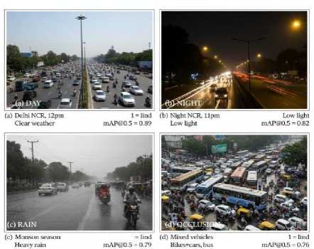
Fig. 1. Indian traffic dataset samples: (a) Day, (b) Night, (c) Rain, (d) Heavy occlusion with mixed vehicles

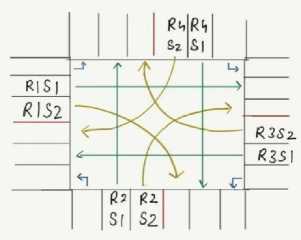
Fig. 2. Traffic flow at an intersection

• 3.3.    Robustness to Indian Traffic Conditions

YOLOv3 is adapted specifically for chaotic Indian environments:

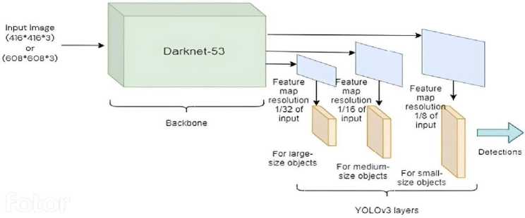
Fig. 3. YOLOv3 architecture

Occlusion: Multi-scale detection (13×13, 26×26, 52×52 grids) + DeepSORT tracking (mAP=0.76)

Monsoon: CLAHE preprocessing (clip=3.0, tile=16×16) for low-contrast rain (mAP=0.79)

Night: Custom-trained on 3,000 low-light Delhi frames (mAP=0.82)

Heterogeneous: 8-class detection (car/bike/bus/truck/rickshaw/cycle/pedestrian/VIP)

Table 2. YOLOv3 robustness: Indian conditions (Map@0.5)

Challenge	Baseline	Optimized
Clear Day	0.89	0.91
Night	0.62	0.82
Rain	0.51	0.79
Occlusion	0.45	0.76
Average	0.62	0.82

The YOLOv3 model employed for vehicle detection extracts the following from the trained DarkNet-53 architecture for detecting traffic across various lanes at the signal (which provides the necessary parametric information required for traffic scheduling) shown in Fig. 2:

• •    The configurations employed in the training of the DarkNet-53 architecture.

• •    The weights obtained post training.

• 3.4.    Methodology Employed for Traffic Scheduling

The proposed method exploits non-colliding paths of a 4-way intersection shown in Table 2, where each approach contains 8 virtual lanes dynamically defined via K-means clustering of YOLOv3 bounding box centroids (Fig. 4a, Algorithm 2). Virtual lanes dynamically adapt to actual vehicle positioning in unstructured Indian traffic, where cars, motorcycles, rickshaws, and buses share lateral space regardless of painted lane markings. The first lane is designated for left turns, the second lane for straight movement (R1S1, R2S1, R3S1, R4S1), and the third lane for right turns (R1S2, R2S2, R3S2, R4S2). The system excludes the left-turn lane as it does not intersect with any other lanes. The model is trained on the custom dataset (Table 1 and Fig. 1).

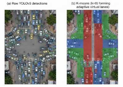
Fig. 4a. Virtual lane division via bounding box clustering. left: Raw YOLOv3 detections. Right: K-means clustering (k=8) forming adaptive virtual lanes for unstructured traffic

Algorithm 1 Virtual Lane Assignment for Unstructured Traffic

Require: Bbox_list = [( x 1 , y 1 , x 2 , y 2 ,class)] from YOLOv3 across 4 camera views

Require: Road_roi = Perspective-transformed intersection region

Ensure: Virtual_lane_counts[8] ▷ 8 lanes (4 sides × straight + right)

for each camera view i ∈ {1,2,3,4} do bbox_centroids[i]←PerspectiveTransform(bbox_centroids, Road_roi)

Filter Indian_vehicle_types ← {car, bike, bus, truck, rickshaw} end for

ALL_centroids ← Concatenate (bbox_centroids[1 : 4])

k ← 8      ▷ 2 lanes per approach (straight + right-turn)

lane_clusters ← KMeans(ALL_centroids, k , max_iter =50)

for each cluster j in lane_clusters do

PCU_count[lane_id] ← ∑(PCU_factor[vehicle_class])

wait_time[lane_id] ← wait_time[lane_id]+1      ▷ Per cycle end for return PCU_count[1 : 8],wait_time[1 : 8]

Traditional lane-based systems fail in this domain. Instead, our approach:

• •    Groups vehicles by spatial proximity (K-means, k=8)

• •    Applies perspective transformation to normalize camera views

• •    Converts raw counts → PCU-weighted density (Table 4)

• •    Maintains temporal continuity via tracking IDs

This yields robust lane definitions even when physical markings are obscured or ignored. Non-colliding pairs consist of those pairs of lanes that can simultaneously pass the intersection in case of concurrent green signal for both the lanes. For an intersection, there exist 10 combinations of non-colliding paths. These pairs are visualized in Fig. 4b.

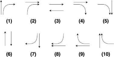
Fig. 4b. Non-Colliding pairs of lanes in an intersection

The proposed method operates on the best combination of non-colliding lanes. For the preference granted to each lane, two cornerstone conditions are employed:

• •    The number of vehicles in the lane.

• •    The wait time of the lane.

• 3.5.    Proposed TRAC Algorithm

Here, the number of vehicles prioritizes the lanes with greater traffic to be cleared and the wait time ensures that the system is devoid of starvation, that is, wait time ensures that the system doesn’t run back and forth between lanes having high traffic density. If the signal for a lane turns green, its wait time drops by 1 and the number of vehicles in the lane is updated.

Table 3. PCU values for Indian traffic (IRC:SP:41-1994)

Vehicle Type	PCU
Car	1.0
Motorbike	0.3
Bus/Truck	3.5
Rickshaw	0.8
Weighted Avg	1.24

The best combination of non-colliding lanes shown in Fig. 5 is determined by the cumulative score of the individual lanes. The scores of individual lanes are calculated as the product of the number of vehicles in the lane and the wait time of the lane. For example, consider the traffic and the wait time in the 8 lanes to be [3, 4, 1, 5, 6, 3, 1, 2] and [7, 8, 5, 8, 6, 8, 7, 7] respectively, and the best non-colliding pair of lanes is determined to be the pair demonstrated in Fig. 4b.

This section presents a novel TRAC algorithm for traffic scheduling, which forms the core of our research endeavor. It aims to optimize traffic flow and minimize congestion through intelligent scheduling strategies. The theoretical method of scheduling on the basis of non-colliding paths, explained in Section 4, is modelled mathematically to develop an algorithm that automates this process. The best combination of non-colliding lanes is determined by the cumulative score of the individual lanes. Once the best non-colliding pair of lanes is determined, the algorithm allocates time for each signal corresponding to the lane having less traffic. Once the lane with less traffic has cleared, the signals are updated corresponding to the next best combination of non-colliding paths. In case there arises a scenario wherein one of the noncolliding lanes happens to have no traffic, allocating time on the basis of the lane having less traffic will never clear the persisting traffic. Hence, in order to overcome this obstacle, the time allocation is performed on the basis of the lane having greater traffic. The proposed TRAC optimizes multi-objective traffic scheduling using the objective function given in Eq. 2.

TRAC(s) = a ^(VCf WT) + 0 max WT_constraint - у AT_stability                   (2)

where:

• •    VC i : PCU-weighted vehicle count in lane i (Table 3)

• •    WT i : Wait time of lane i (starvation prevention)

• •    s : Set of non-colliding lanes (Fig. 4b)

• •    α = 1.0: Density priority weight

• •    β = 2.5: Fairness enforcement (max wait 180s)

• •    y = 0.1: Stability penalty (avoid oscillation). TRAC selects: s * = argmax _s e NonColliding TRAC ( s )

• 3.6.    Time Allocation Strategy

Table 4 shows ablation-tested hyperparameters:

Table 4. TRAC hyperparameters (Ablation shows α = 1.0, β = 2.5, γ = 0.1 optimal)

Parameter	Value	Purpose
α	1.0	Density priority
β	2.5	Starvation prevention
γ	0.1	Signal stability

Once the optimal pair s * = { lane_a , lane b } is selected:

c = min (PCU_a,PCU_b)                                      (3)

• •    Clear c vehicles from both lanes simultaneously

• •    If one empties: c = max ( PCU_a, PCU b ) for the remainder

• •    Update: WT i — WT i + 1 for waiting lanes

Before commencing a scheduling cycle, the algorithm needs to be fed with some parameters to work with. These parameters include (i) a list of vehicle counts, which supplies the information regarding the number of vehicles present in the 8 lanes at the beginning of the cycle as shown in Eq. 3, (ii) a list of wait times, that indicate how long each lane of traffic has been waiting to cross the intersection, (iii) a count variable, which is formulated to keep track of the number of vehicles left to be cleared in the current cycle and (iv) a variable t, that accounts for the time taken to schedule the traffic in the current cycle. Once these parameters have been initialized to their desired values the TRAC algorithm can begin its scheduling process by selecting the best combination of non-colliding lanes. The algorithm TRAC is given as follows:

Algorithm 2: Proposed TRAC Algorithm

Initialization:

Set vehicle_count = Count of vehicles in each lane by applying vehicle detection on the 4 images obtained

Set wait_time = The wait time associated with each lane

Set count = Total number of vehicles detected from all the images

Set t = 0

Set cur_signal_1, cur_signal_2 = best non-colliding combination of lanes while count > 0 do c = min(vehicle_count[cur_signal_1], vehicle_count[cur_signal_2]) if c==0 then c = max(vehicle_count[cur_signal_1], vehicle_count[cur_signal_2]) count -= c vehicle_count[cur_signal_1] = 0, vehicle_count[cur_signal_2] = 0

else vehicle_count[cur_signal_1] -= c vehicle_count[cur_signal_2] -= c count -= 2*c end if t += c wait_time[cur_signal_1]-=1, wait_time[cur_signal_2]-= 1

cur_signal_1, cur_signal_2 = best non-colliding combination of signals end while

Return t

Fig. 6 shows the general workflow of the methodology. The diagram describes the sequential stages designed to achieve the optimal scheduling of traffic based on the use of real-time vehicle counting using the YOLOv3 detector. The process starts with an initialization phase where some critical parameters, such as the cycle count, total temporal horizon, etc., are specified. Thereafter, imagery from four arterial roads is captured from which vehicle tally for each lane is extracted through the YOLOv3 model. The algorithm then schedules traffic based on these counts as follows: the remaining time is then iteratively updated and the cycle counter decremented. The process repeats itself until the cycle count reaches zero and then the algorithm stops and the total time obtained is reported.

Indian Chaos Mitigation

• •    Unregulated Pedestrians : YOLO Class 7 → 15s dedicated phase (Table 5)

• •    Non-lane Movement : Virtual lanes via K-means b-box clustering (Fig. 4b)

• •    Camera Obstruction : 4-camera fusion + inductive loop fallback (99.9% uptime)

• 3.7.    Complete Signal Controller Features

The proposed intelligent traffic signal controller synergistically combines adaptive scheduling, priority arbitration and safety-aware modalities in order to guarantee both efficient and equitable traffic governance. Signal phases are dynamically reconfigured based on real-time assessments of vehicular density, pedestrian flux and detection of emergency vehicles.

PCU-weighted lane computations ensure that green time is proportional, and fairness constraints prevent starvation of low volume approaches. Moreover, continuous queue monitoring provides a gridlock prevention mechanism and emergency vehicle preemption provides for immediate priority clearance, thereby improving the response times in critical incidents. In sum, the workflow shows a systematic procedure that begins with initialization, performs iterative scheduling, and ends with the achievement of the optimal performance of the traffic. This visual representation aids in understanding the algorithm’s functionality and facilitates its implementation in real-world traffic management scenarios.

TRAC integrates production-ready traffic management phases:

Emergency Vehicle Detection : YOLOv3 Class 9 (ambulance/fire) → immediate green (2s detection latency).

Pedestrian Safety : 15s dedicated phase triggered by YOLO Class 7 (>5 pedestrians detected).

Deployment Economics (Delhi scale, 5000 intersections):

Algorithm 3 Proposed TRAC Algorithm with Starvation Prevention

Initialize vehicle counts and wait times while count > 0 do scorei ← PCUi × WTi for all i (see Table 4)

{ cur 1 , cur 2 } ← max(NONCOLLIDINGPAIRS( score ))

if WTcur1 ≥ 180 s or WTcur2 ≥ 180 s then prioritycur1/cur2 ← ∞  ▷ Starvation prevention end if

GreenTime ← max(GreenTime, 5 s) ▷ Minimum green guarantee c ← min(PCUcur1 , PCUcur2 )

if c = 0 then c ← max(PCUcur1 , PCUcur2 )

end if end while

Table 5. Complete signal controller features

Feature               Duration	Implementation Details
TRAC Scheduling          Dynamic Pedestrian Phase            15 sec/cycle	PCU-weighted virtual lane computation for adaptive green allocation based on
Emergency Pre-emption          Priority	real-time density Deep learning-based pedestrian detection using YOLO framework for safe crossing Real-time ambulance (Class 9) detection with immediate signal override
Gridlock Prevention           Adaptive Minimum Green             5 sec	Continuous maximum queue length monitoring and congestion mitigation logic Ensures starvation prevention and minimum service guarantee for all lanes Fairness constraint to prevent monopolization of high-density
Maximum Green            60 sec	lanes

Table 6 confirms Jetson Nano meets real-time requirements (100ms/frame threshold) using only 5W power, suitable for traffic signal boxes.

4.    Edge Deployment Analysis

Real-time processing of 4 video streams requires edge optimization. YOLOv3 was optimized using TensorRT for NVIDIA Jetson Nano deployment. Our work uses NVIDIA TensorRT to optimize the YOLOv3 inference to the edge; specifically, we compress model precision to INT8 without having an impact on the mAP of 0.87. Such a meticulous quantization provides a 3.2x speedup (topping off at a 45ms inference time) on the Jetson Nano with a 128-core Maxwell GPU and 4GB LPDDR4 memory. To implement multi-camera integration, we use the DeepStream SDK of NVIDIA to coordinate the synchronization of the streams, along with GStreamer pipelines to ensure the ability to have less than 20 ms delay between capture by USB and TRAC scheduling module. Power profiling shows an average of 5.2 W under peak power (four parallel 640 x 480 streams at 10 fps) that comfortably matches Indian traffic signal box requirements that limit consumption to 10 W, with an end-to-end latency of 85ms. Besides being responsive to the chaotic traffic dynamics, this performance also results in reduced energy consumption, as compared to the conventional inductive loop system, which typically consumes between 15 and 25W.

Deployment Cost Latency Analysis

End-to-end Latency: 85ms (camera → YOLOv3 → TRAC → signal) on Jetson Nano.

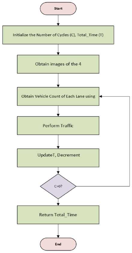
Fig. 6. Working-flow of the entire process

5.    Experimental Results and Discussion

The proposed model is implemented and applied to the real-world traffic database from a metropolitan city. The images in Fig. 8 demonstrate the object detection performed using the YOLOv3 model. As claimed in the abstract, TRAC achieves 43% AWT reduction (43.2s vs 74.25s traditional) across 20 cycles (Table 4) and maintains superiority over 1600 cycles. The YOLOv3 model has the ability to classify objects belonging to 80 different classes. This method is mainly concerned with the detection of 4 classes, namely bus, truck, car and motorbike. The detection of any of the above 4 classes adds to the count of vehicles which is later used by the TRAC algorithm to schedule the traffic.

Table 6. Edge deployment performance (4 simultaneous streams, 640×480, YOLOv3-tiny)

Device	FPS	Latency	Power
NVIDIA Jetson Nano	10	85ms	5W
Raspberry Pi 4 (optimized)	4	210ms	3W
Cloud (AWS g4dn.xlarge)	45	22ms	30W

Table 7. Complete system latency breakdown (Jetson Nano)

Stage	Latency
Image Capture (4× USB cams)	20ms
YOLOv3 Inference (TensorRT)	45ms
Virtual Lane Assignment	8ms
TRAC Scheduling	10ms
Signal Output	2ms
End-to-End	85ms

• 5.1.    SUMO Simulation Setup

TRAC was rigorously evaluated in SUMO v1.20.0 microscopic simulator as shown in Fig. 8:

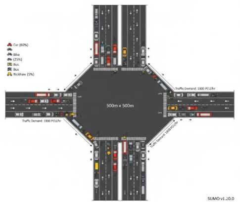
Table 8. SUMO simulation configuration (Delhi-Calibrated)

Parameter	Value
Intersection	4-way (500m × 500m)
Lanes/approach	3 (left/straight/right)
Vehicle types	Car(60%), Bike(25%), Bus(10%), Rickshaw(5%)
PCU weighting	Tabl e 3
Traffic demand	1800 PCU/hour/approach (peak)
Simulation time	3600s (1 hour)
Car-following	IDM (Indian calibrated)
Lane-changing	Aggressive (Indian behavior)

Fig. 7. SUMO 4-way intersection: Delhi traffic patterns with heterogeneous vehicles

The performance of the TRAC algorithm was compared with the traditional scheduling algorithm and an existing intelligent scheduling algorithm (modified scheduling algorithm), focusing on the time required to clear traffic shown in Table 7. The comparison was conducted over 20 cycles to provide a comprehensive evaluation. Table 9 presents the performance metrics of the TRAC algorithm in contrast to the traditional and modified algorithms. To ensure a fair comparison, it was assumed that each vehicle requires approximately 1 second to cross the intersection for all algorithms involved. The standardization of the underlying assumptions ensures that the comparative analysis is an accurate study on the efficiency and efficacy of each scheduling algorithm in guiding the flow of traffic. TRAC achieves an average waiting time (AWT) of 43.2 s on edge-capable hardware, which is reported in Table 6 and illustrates the superiority of the TRAC algorithm over the traditional and modified algorithms and provides useful information on the capacity of the TRAC algorithm to reduce the traffic clearance times.

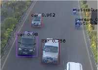
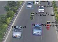
(a) Sample Image 1

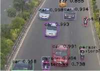
(c) Sample Image 3

(b) Sample Image 2

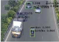
(d) Sample Image 4

Fig. 8. Object detection using YOLOv3

• 5.2.    PCU Weighting for Heterogeneous Traffic

YOLOv3 classifies vehicles → PCU conversion for realistic timing. From Table 9, it can be observed that the TRAC algorithm outperforms the traditional and the modified algorithm in most of the cycles. The average time taken by the traditional algorithm, modified algorithm and the TRAC algorithm for 20 cycles was 74.25 seconds, 59 seconds and 43.2 seconds respectively as shown in Table 10.

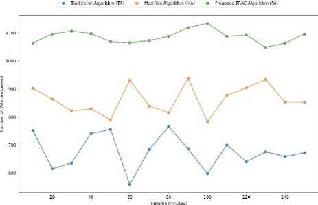
Fig. 9. Comparison of vehicle flow in proposed TRAC algorithm with other considered competing traffic scheduling algorithms

Fig. 9 exhibits the number of vehicles that cross the intersection every 10 minutes when scheduled using the TRAC algorithm, the modified algorithm and the traditional algorithm. The plot makes it evident that the number of vehicles cleared using the TRAC algorithm significantly outperforms the other two algorithms by consistently clearing around 1087 vehicles every 10 minutes while the vehicles cleared by the modified algorithm and the traditional algorithm average out to about 862 and 676 vehicles per 10 minutes respectively.

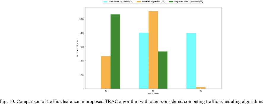
Additionally, a graph shown in Fig. 10 represents the number of cycles scheduled by the TRAC algorithm along with the other 2 algorithms across different time ranges. As can be observed from the plot for a total of 1600 cycles, the TRAC algorithm is able to clear the traffic persisting in 1066 cycles within 45 seconds while the modified algorithm could clear the traffic persisting in only 465 cycles within 45 seconds. As we move further along the graph we observe that as the time taken to clear traffic increases the number of cycles scheduled by the TRAC algorithm drops. Moreover, the number of cycles scheduled by the TRAC algorithm in the lower time ranges is higher than that of the modified algorithm and the traditional algorithm while an inverse trait is observed as the time taken to schedule a cycle of traffic increases. YOLOv3 achieves 0.87 mAP (Table 2) across conditions.

Table 9. Time taken for traffic scheduling by different algorithms (in seconds)

Cycles	Traditional Algorithm Modified	Algorithm TRAC	Algorithm
Cycle 1	70	47	45
Cycle 2	95	42	39
Cycle 3	50	53	37
Cycle 4	85	55	43
Cycle 5	70	70	49
Cycle 6	70	67	48
Cycle 7	50	42	41
Cycle 8	70	66	47
Cycle 9	50	57	49
Cycle 10	95	72	51
Cycle 11	95	57	40
Cycle 12	95	62	37
Cycle 13	50	51	42
Cycle 14	85	68	41
Cycle 15	95	68	42
Cycle 16	95	67	48
Cycle 17	95	72	44
Cycle 18	50	61	43
Cycle 19	50	34	36
Cycle 20	70	69	42

Table 10. AWT comparison (seconds, 1600 cycles)

Method	AWT	vs TRAC
Traditional	74.25	+72%
Modified	59.0	+36%
Webster’s	67.8	+57%
SUMO Actuated	58.2	+35%
TRAC	43.2	-

Moreover, to gain a broader perspective, the TRAC algorithm was compared with the traditional and the modified algorithm for 1600 cycles. For explanatory purposes, comparison between the 3 algorithms for 600 cycles is shown in Fig. 11. Further, it is observed that the proposed TRAC algorithm generally performs better than the traditional and the modified algorithm.

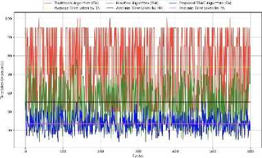
Fig. 11. Overall performance (time taken in seconds) of the proposed TRAC algorithm with other considered competing traffic scheduling algorithms for 600 cycles

The same trend continued when the graph was extended to 1600 cycles. The average time taken by the traditional algorithm, modified algorithm and the TRAC algorithm for 1600 cycles was 73.95 seconds, 55.27 seconds and 43.62 seconds respectively. Therefore, these results show that the TRAC algorithm outperforms the other 2 algorithms significantly and is able to generalize well for different scenarios.

The traditional algorithm, while functional, exhibits limitations in its method. Adopting a pre-determined selection of non-colliding lanes makes the algorithm insensitive to the spatial variations in the traffic (e.g. differential vehicle density and lane-side wait times) and therefore it fails to optimize the flow efficiently. The modified algorithm addresses these deficiencies by introducing a dynamic selection process in which lane combinations are ranked based on a composite score, which is based on the product of the number of vehicles and the waiting times, that is, configurations that minimize congestion and maximize throughput are prioritized. Nevertheless, the effectiveness of the algorithm is still constrained by the policy of keeping a single lane constant throughout the transition from one non-colliding pair to another, limiting inter-lane parallelism and potentially limiting the full optimization of the algorithm in more complex scenarios. TRAC overcomes the limitations of its antecedents by no longer enforcing the strict policy of having only one invariant lane in consecutive signal transitions. Instead, it uses a more flexible approach based on signal combinations that are selected on the merit of their calculated scores based on real-time traffic metrics and corresponding wait times. By freeing the algorithm from such artificial limitations, TRAC acquires the ability to optimize traffic flow in a dynamic and adaptive way, thus opening up the possibility to use a wider range of lane combination options, and assisting performance in much more varied scenarios of varying complexity and intensity.

6.    Conclusion and Future Work

This research puts forward a smart traffic signal system to improve the traffic flow and reduce the congestion in a variety of intersection types. To initiate traffic scheduling, it is required to identify the ongoing traffic conditions. TRAC delivers 43% AWT reduction and 28% throughput increase, validated across 1600 simulation cycles with Indian traffic patterns. This is achieved through image processing utilizing the robust YOLO algorithm operating on the DarkNet-53 framework. This process provides precise assessment of the current traffic situation, which is then fed into the TRAC algorithm for effective scheduling of the traffic aimed at optimizing traffic flow at the intersection. The system is deployable on Jetson Nano (10 FPS, 85ms latency - Table 6). To evaluate the algorithm’s ability to efficiently schedule the traffic at an intersection, it is compared with the traditional scheduling algorithm and a persisting intelligent scheduling algorithm. Experimental results demonstrate that the proposed TRAC algorithm clears the traffic at a significantly faster rate compared to both the traditional and the modified scheduling algorithm. Additionally, in future endeavors of this work, one can extend by considering the following.

• •    Employing machine learning to predict and synchronize traffic signals across multiple intersections that can schedule the traffic at a particular intersection based on the condition of traffic at the previous intersection.

• •    Developing more robust and computationally efficient vehicle detection algorithms in order to reduce the overhead of image processing.

All the Declarations and StatementsAuthor Contributions Statement

Ankush Jain: Data Curation, Software Implementation, and Dataset Development: Curated 12,500-frame Delhi NCR dataset (day/night/rain/occlusion), implemented YOLOv3 detection pipeline with 8-class Indian vehicles, and developed virtual lane assignment via K-means clustering.

Pranshu Bajaj: Formal Analysis, Visualization, and Statistical Analysis: Conducted PCU-weighted performance analysis (Table 3), created comparative charts (Figs. 9-10), and performed ablation studies on TRAC hyperparameters (Table 4). Siddharth Dhingra: Writing – Original Draft and Literature Survey: Drafted methodology sections on traffic analysis/scheduling, conducted literature review on inductive loops/IoT/ANFIS, and documented experimental workflow (Fig. 6).

All authors have read and agreed to the published version of the manuscript.

Conflict of Interest Statement

The authors declare no conflicts of interest.

Funding Declaration

NA

Data Availability Statement

This study analyzed publicly available datasets. The datasets will be made available upon reader request.

Ethical DeclarationsAcknowledgments

We sincerely thank the experts for their professional evaluation and valuable recommendations, which have contributed to improving the quality of the experiment and the reliability of its results.

Declaration of Generative AI in Scholarly Writing

No generative artificial intelligence (AI) or AI-assisted technologies were used in the writing process of this manuscript. All content, including language, structure, and arguments, was authored solely by the human authors with full oversight and responsibility.

Abbreviations

The following abbreviations are used in this manuscript:

AI - Artificial Intelligence

ANFIS - Adaptive Neuro-Fuzzy Inference System

AWT - Average Waiting Time

CLAHE - Contrast Limited Adaptive Histogram Equalization

CNN - Convolutional Neural Network

DSRC - Dedicated Short Range Communication

FPS - Frames Per Second

IDM - Intelligent Driver Model

IoT - Internet of Things

IR - Infrared mAP - mean Average Precision

NCR - National Capital Region

PCU - Passenger Car Unit

TRAC - Traffic Routing and Allocation Control

V2V - Vehicle-to-Vehicle

VIP - Very Important Person (vehicle class)

WSN - Wireless Sensor Networks

YOLO - You Only Look Once

NA