The climatic conditions of the Arctic and new approaches to the forecast of the climate change

The northern regions of the Earth play a significant role in the processes that affect on the environment on a global scale, and serve as indicators of the global natural changes, particularly climate changes. The changes observed in the Arctic, such as the increase of the temperature, the reduction of the ice cover, increase of river flows and degradation of permafrost, already show that the biggest changes occur in the territory of the Arctic in comparison with other regions of the Earth.

In the current strategy of development of the Russian Arctic one of the priority guidelines is the integrated socio-economic development of the region1. Harsh climatic conditions of the Arctic greatly hinder the forming of infrastructure there and development of discovered large reserves of mineral resources in the Arctic. At the same time the largest and currently the hidden problem is climate change and the uncertainty of its future condition. The successful development of the Arctic zone is impossible without reliable forecasting climate estimations for several decades in advance.

In all the Arctic countries exploration plans of the Arctic zone are based on the realities of today's abnormally warm climate, during the period of the global warming, in conditions of reduction of the ice cover and opening of the Northern Sea Route and the West Passage, and also on the basis of assumptions about the further global warming.

In fact, we know a little about future climate of the Arctic region. This is due to our lack of knowledge about the reasons of modern changes of global climate and in connection with the special conditions of climate formation in the high latitudes of the Earth, which complicate the forming of reliable forecasts of the future state of the Arctic climate.

High latitudes of the Earth, the Arctic are the unique region in terms of formation of the temperature. The first feature — the Arctic climate is formed in much smaller inflow of heat from the sun than the climate of non-polar regions. On Earth, to the north of 70° latitude the sun does not appear for several months (polar night) and during few months it does not go beyond the horizon (polar day). Highly reflective ability of snow and ice, as well as predominantly low height of the sun above the horizon do not allow the temperature to form the temperature baseline which is observed in the Arctic. Heat of the Arctic region is largely determined by amount of the advective ending brought by ocean currents and air streams from the low latitudes. The amount of advective ending in the Arctic depends on the global oceanic and atmospheric circulation processes. The second feature of the Arctic — this is a region with climate most sensitive to changes in amount of so-called greenhouse gases in the atmosphere (water vapor, carbon dioxide, methane, etc.) and the amount of cloud cover. Radiation balance at high latitudes is preferably negative, and temperature conditions are mainly determined by the ability of the atmosphere to prevent emission of heat to go to space of coming advective ending. In middle and low latitudes, the situation is different, there the temperature mode is determined primarily by the amount of incoming solar radiation to the surface of the earth, and depends less on the greenhouse effect. In the process of anthropogenic increase of greenhouse gases in the atmosphere this feature of the Arctic has a particular importance. The third feature — near the geographic pole there is geomagnetic pole, which creates at high latitudes favorable conditions for the invasion of charged solar and cosmic particles. The intensity of the flow of these particles depends on the variable solar activity. There are many publications over the past few decades confirming connection of weather and climate changes with variable particle flows during change of solar activity, but the mechanism of this connected is not explained.

The Arctic climate changes are strengthened by feedback connections, the degradation of the sea ice in the Arctic Ocean, sensitive to climate changes, attracts special attention. Removal of fresh water from the Arctic Ocean influnces upon the expansion of sea ice, thermohaline circulation in the adjacent waters of North Atlantic and through them to the regional and global climate. Presence of several variable heat sources, as well as feedback connections between them makes the Arctic as region of greatest changes and climate variability. Many features of interrelated processes remain poorly explored.

Climate changes

For a long time in the modern history climate was considered unchanged in nature. But in the 1920s many reports about signs of warming in the Arctic came out. Knipovich N.P in 1921 said that the Barents Sea waters became noticeably warmer [1, p. 10-12]. At first it was considered that the warming is related only to the Arctic region. Later it was noted that it was global warming. A feature of warming was the fact that at high polar latitudes of the Northern Hemisphere it was expressed more clearly and vividly. For example, in West Greenland temperature increased by 5 °C, and at Spitsbergen even by 8-9 °C for the period of 1912—1926 to until the end of the 30s. The greatest increase in average global temperature near the Earth's surface during the highlight of warming was 0.6 °C. The Arctic was figuratively called the "weather kitchen".

After the 1940s the tendency to cooling started to appear. The ice in the Northern Hemisphere began to attack again. It was mainly reflected in the growth of the ice cover area of the Arctic Ocean. Since the beginning of the 40's and until the end of the 60’s the ice area in the Arctic basin has increased by 10%. The first warming gave way to brief and gentle cooling in the middle of the XX century.

Since the middle of 1970s the second glabal warming in the history of instrumental observations started, and it received very different explanation connected with strengthening of greenhouse effect from anthropogenic increase of the concentration of carbon dioxide and other greenhouse gases in the atmosphere.

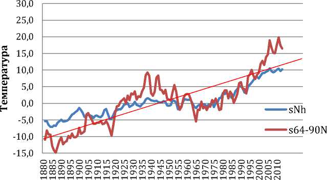
Fugure 1. Air temperature in the Arctic at 64-90 ° north latitudes in the northern Hemisphere.

In Figure 1 two waves of woarming can be seen: first in the 1930s and the second since 1970. But in some authoritative publications the mere appearance of the second wave of global warming was disputed for a long time, until the early 1990s, when the fact of global warming has become generally accepted.

And the hypothesis of anthropogenic warming became the main one. After accept of anthropogenic hypothesis the prognostic scenarios of expected one-directional and inevitable catastrophic climate changes appeared by the end of the XXI century. Such scenarios are still considered the main ones. However, starting from the beginning of the XXI century the global warming was suddenly changed by the so-called pause in warming — increase of global temperature stopped, as it was earlier in the peak of first global warming in 1930—1940s. The problem was especially acute if we observed the change or variation of climate?

Instrumental observations of temperature appeared preferably not earlier than the end of the XIX century, but in central England the information about the temperature are known from the XVII century. According to these data long-term variations of temperature always happened.

For example, temperature in central England before the pre-industrial era in XVII—XIX centuries, three full waves of century variations were observed, and in the second half of XX century the phase of 4th wave of warming started, but after that there was a pause that lasted for more than 15 years.

What will be next? If to extrapolate the natural fluctuations in coming decades, then the transition to the phase of decrease of temperature can be expected, and if anthropogenic hypothesis is correct, then the warming continues.

According to satellite observations since the second half of XX century till the present time, the highest temperature of the troposphere of the northern hemisphere was observed in 1998, and then there is a pause. It is important to compare the regional features of the climate changes until 1998 and later. We calculated the value of the coefficients of the linear approximation (linear trends) of changes in air temperature over land and ocean surface temperature for two separate periods of time for 1976—1998 and 1999—2014 years. Calculations were made according to observations at meteorological stations in the northern hemisphere and to the values of ocean surface temperature in the geographical grid centers of 5x5 degrees. In period of 1976—1998 years the warming was observed in the whole territory of the northern hemisphere. In large areas, mostly over land, the greatest warming was 1,5÷2,0оС/10 years. After 1998, there was a pause in global warming, the temperature increase was only in the Russian part of the Arctic and in

Greenland area. But a decrease in temperature occurred in the Canadian Arctic for the last 16 years.

This development of events is not consistent with predictive scenarios of climate change, based on physical and mathematical climate models [2], which are often presented as the most complete and reliable for estimates of future climate. These models are based on the assumption about greenhouse nature of modern climate changes under increasing anthropogenic greenhouse gases in the atmosphere. Other possible factors of climate changes were not taken into account in these models due to lack of understanding of the mechanisms of their impact on the climate. But there are many publications, in which the external factors are considered.

Reasons of climate changes

The problem of reasons of the modern climate changes remains disputing. At the present time only four possible factors of modern climatic changes occurring in the global and regional scale are accepted more often:

• a.    Anthropogenic effects of greenhouse gases — the main factor.

• b.    Increasing the flow of incoming solar radiation (usually ignored).

• c.    Reducing of the role of aerosol scattering.

• d.    The internal fluctuations of the climate system consisting of the atmosphere, ocean, hydrosphere, land and cryosphere (ignored or treated as a minor factor).

Regional changes in air temperature are always connected with changes in atmospheric circulation. Changes in the general circulation of the atmosphere are often considered as a climate factor. Atmospheric circulation not only redistributes heat around the planet, but also creates such new conditions in the global atmosphere, which are accompanied by fluctuations in the global climate. Changes in atmospheric circulation can be long — of climate scale, so the atmospheric circulation can be considered as a factor of climate. But here the question about the reasons of change of the atmospheric circulation arises. In the atmospheric circulation natural oscillations as well as changes or fluctuations under the influence of external factors can be present.

The warming of 30s of XX century came in history as the "warming of the Arctic," was associated with an increase of duration of the zonal circulation. The increase of the total length of the Atlantic cyclones moving along the coast of Eurasia contributed to increase of the air temperature in the coastal weather stations in the Arctic basin and in the temperate latitudes. Maximum duration of zonal circulation was observed in the decade of 1931—1940. These are the first years of the global warming.

The second global warming begins from the 1970s and is well coordinated with increase of length of the group of circulation with cyclones at the poles. With these macroprocesses in the northern and southern hemispheres cyclones come from low to high latitudes, which is accompanied by increase of the temperature in the middle and high latitudes.

The first warming was zonal and most evident at high latitudes. The second warming was more spreading in different latitudinal zones. It reached the peak in 1998. Cooling began after duration of circulation group with cyclones at the poles reached maximum in 1997.

The observed current climate changes are well coordinated with the rearrangements in the general circulation of the atmosphere. Kononova N.V [3, p. 11—35] found that changes in the average global temperature during the XX century — beginning of the XXI century are in antiphase with the changes of the summary annual length of the blocking processes and in phase with the duration of a particular type circulation on the poles. Currently there is increase of duration of the blocking processes [3, p. 11—35] and observed decrease in ocean surface temperature [4, p. 98— 104] contributing to a further reduction in global annual average air temperature.

Disturbances in the atmospheric circulation may be the result of forced or natural oscillations in the climate system under the influence of external forcing fluctuations or episodic external impacts.

The atmosphere is less inert component of the climate system and is subject to multifactorial influences in the process of interaction with other components of the climate system as well as under external factors. Because of the low thermal inertia of the atmosphere, long-term processes in it can only be formed under the influence of external energy sources.

The closest source of long-period atmospheric disturbances is heat exchange: ocean — atmosphere and ocean circulation processes. Academician Monin A.S pointed out that the climate is formed under the influence of number of factors, which can be divided into three groups:

• a.    External or astronomical factors — the luminosity of the Sun, the position and moving of the Earth in the solar system, the inclination of the Earth's axis to the orbit plane and the speed of axial rotation, determining the impacts on the planet by other bodies in the solar system, its insolation and gravitational effects of the external bodies, creating tides and fluctuations of the characteristics of the orbital motion and proper rotation of the planet;

• b.    geophysical and geographical factors — number of features of the planet, from which the most important for the Earth's climate are the properties of the underlying surface, which define its thermal and dynamic interaction with the atmosphere;

• c.    atmospheric factors — the mass and composition of the atmosphere.

Perhaps the list of these known and suspected factors of the climate changes is not complete.

Anthropogenic warming factor . In recent decades the largest attention was paid to anthropogenic change in atmospheric composition as a possible factor of the strengthening of the greenhouse effect of the atmosphere and global warming in the second half of the XX century. In the publications of the Intergovernmental Panel on Climate Change (IPCC) the conclusion was made about the anthropogenic nature of the modern warming connected with increasing concentrations of CO 2 , methane and other greenhouse gases in the atmosphere: “With a high degree of certainty it is possible to confirm that the observed increase of the anthropogenic greenhouse gas causes a major part of the global warming of the second half of XX century. Carbon dioxide through the greenhouse effect in the atmosphere makes the main contribution to global warming” [2]. Judging by the large number of publications, the output obtained on the basis of model estimates was received that the rapid growth of greenhouse gas emissions is a result of the intensification of human activities. As before and especially recently, more and more publications appear in which the alternative hypotheses are offered.

IPCC conclusions are based on estimates received from the physical and mathematical modeling on the assumption that the models take into account all factors and adequately reflect all the processes with their multilateral and direct feedback connections for all components of the climate system. Though it is certainly known that the models are far from being perfect. The first doubt in the unconditional anthropogenic nature of the modern warming is based on historical facts about the climate in the past, according to which these and stronger warmings were observed many times in the past and then each time later they were followed by coolings. It happened in the pre-industrial era.

According to the academician Kotlyakov V.M. data, concentration of greenhouse gases and global temperature in the past varied concurrently, as it follows from the analysis of ice cores for a few centuries, and the level of gases in the atmosphere really increased dramatically over the past 100 years, but recent changes in temperature do not go beyond its natural historical fluctuations in the pre-industrial era. The concentration of CO 2 in the atmosphere is subject to natural fluctuations. According to known laws of physics, depending on the upper ocean temperature, CO 2 is heavily disolved in the ocean during colling or released from the ocean into the atmosphere during warming. According to these data, the change of CO 2 concentration in the atmosphere can be regarded as a consequence of warming but not as its reason.

According to data of academician Nigmatulin R.I. [5, p. 1—8] values of natural CO2 flows from the ocean into the atmosphere and from the atmosphere to the ocean are many times greater than the CO2 emissions resulting from human activity. Can we be sure that the existing imperfect ocean models with such comprehensive accuracy describe the state of the upper layer of the ocean, in order to properly estimate the balance of the natural long-term fluctuations of CO2 concentration and evaluate the impact of the exclusively anthropogenic CO2 additive in climate change? Recognizing the anthropogenic component in current climate changes, we can not reject the existence of natural climate variabilities which always took place and still exist.

According to opinion of academician Kotlyakov V.M. [6, p. 44—47], " No matter what anthropogenic climate changes are , they are superimposed on its natural variations, the scale of which is still greatly exceeds the impact caused by greenhouse gas emissions… Understanding and prediction of the effects of increase of the greenhouse gases in the atmosphere (so-called global warming due to the greenhouse effect) requires an understanding of the natural variability of natural processes on which human influence is overlapped. "

According to observations at fifteen hundred Russian meteorological stations by the author [7] the research of contribution of increase of CO2 concentration in the second half of the twentieth century in changes of the air temperature was carried out. Statistical experiments were made in which the influence of heat advection, the greenhouse effect of water vapor and clouds in the air temperature changes at different latitudes and in different seasons were leveled out, and dependence of the remaining changes in temperature from radiation balance of the earth's surface was estimated. After excluding these natural factors, changes in temperature and radiation balance could occur, mainly due to changes of CO 2 concentration in atmosphere. It turned out that share of CO 2 in total temperature variability was about 25%. These observations confirmed the influence of increased concentrations of greenhouse gases on the climate, but at the same time demonstrated that the assessments of physical and mathematical models of the dominant role of the increase of greenhouse effect in climate warming in the second half of the twentieth century were too much overreported.

Solar Activity . The Earth's climate is primarily the result of the impact of solar energy in existing astrodynamics parameters of the Earth. Therefore, the first two terms of the constancy of climate are to keep the luminosity of the Sun and Earth's orbit parameters. In fact, neither one nor the other remains strictly constant, there are small variations. At the beginning of the 1980s the variability of the solar constant was discovered with an amplitude of 0.1-0.2%, related to the 11-year solar cycle. Reduction of the solar constant is connected with appearance of very large sunspot groups in the Sun, and slight increase — with solar torches. If solar activity is high, the number of spots (sunspots — dark formations) on the Sun increases, the solar constant to some extent depends on area of them. Appearance of sunspots and torches in the Sun disc explains only

50-70% of the observed variations in the solar constant. Possible reasons for the cyclic variability of the solar constant may also be changes in the Sun's diameter. According to data of Abdusamatov Kh.I., [8], changes in the solar constant are 0.07%. The effect of such small variations in the solar constant remains controversial and is reduced to the question of the sensitivity of the climate system to such variations.

The phenomenon called as changes in solar activites are not limited by changing the luminosity of the Sun. The sun is also a source of streams of charged solar particles and modulator of cosmic ray flows that affect the magnetosphere and upper atmosphere of the Earth, especially in high latitudes, and are able to create a disturbance in the atmospheric circulation with consequences for weather and climate.

Astrodynamics factor. The amount of radiation absorbed by the Earth's surface plays also important role in climate variations. From the astronomical point of view, the absorption of Solar energy by the Earth is determined, above all, by the angle of incidence of sunlight to the surface of the Earth, which depends on the angle of inclination of the Earth's axis to the ecliptic. As a result of the interaction of the Earth with the Moon and planets the variations in the parameters of the orbital motion of the Earth and tilt of the Earth's axis arise. At this the conditions of solar radiation absorption are changed, as well as the duration of the seasons and, therefore, the total annual influx of solar heat in the climate system. Astrodynamics conditions are the basis of the formation of the radiation of the planet's climate components. Variations in the parameters of the orbital motion of the Earth and the tilt of the Earth's axis may be accompanied not only by radiation but also dynamic perturbations in all shells of the Earth. The Earth is always experiencing recurring variable gravitational effects from other bodies in the Solar system. As a result of these actions components of the Earth's movement never remain constant. Disturbances can vary greatly in value and have different temporal scale from a few days up to many thousands of years. The values of the perturbation parameters of the Earth’s motion depend on the mass of the perturbing bodies and the distance from them to the Earth. That is why the strongest perturbations are determined by closest bodies such as the Moon, Venus, Mars, and massive Jupiter. Influence of the huge Saturn is weaker due to its great remoteness.

The gravitational interaction of the Earth with the planets and the Moon creates variations in the Earth's orbital velocity, in the north-south and radial deviations from normal orbit, creates precession and nutation of the Earth's axis, changes the Earth's rotation around its axis. In the process of interaction, the distance from the Earth to the sun is changed. These are the parameters which define the space (main) part of processes that form the Earth's climate. The question is whether these variations are so essential to significantly influence on the Earth's climate fluctuations.

Resonances in sun and climate systems . The climate system in all its parameters is manifested as a complex oscillatory system with many nonlinear interactions. For millions of years the climatic oscillatory system has passed a few stages of the evolution. Regardless of its nature, nonlinear oscillatory systems during the dynamical evolution tend to go on a special synchronous drive mode. From the theory of vibrations, it is known that the collection of isolated objects vibrating with different frequencies, when applied with very weak bonds, go into such driving mode in which the frequencies of the objects become equal, divisible or being in rational ways. In synchronization process beside commensuration of frequencies also certain phase relationship between the oscillations are set. [9, p. 34—48].

During the synchronization process certain phase relationship between the oscillations are set besides commensurability of frequencies [9, p. 34—48]. Commensurabilities between the frequencies are very common in the real solar system. The hypothesis about the resonant structure of the solar system is the part of the general theory of behavior of complex oscillatory systems. Resonances may occur in the fluctuations of characteristics of the climate system. In this case they may become the basis of rhythms of different duration and frequency in the climate system, as well as the reason of long-term changes in the climate system parameters (hypothetically could be one of the causes of climate variability).

During the study of the evolution of nonlinear vibration systems, it is necessary to take into account dissipative forces existing in real conditions. These forces are directed to neutralize the interacting vibrations, chaotic to each other. But these same forces lead to the resonant amplification of the oscillations, which are interconnected in judicious mix. Forces of interactions may be more or less (speed of evolution depends on their values), speed of way out of the system into stationary resonant mode depends on it. The final stationary state of the system, achieved by end of the evolution, have to be resonant. Evolutionary mature oscillatory systems are inevitably resonant, and their structure is set, like quantum systems, by set of integers. In real time dissipative forces can be ignored, but in the evolutionary time scale cumulative effects of small dissipative forces become determine [9, p. 34—48].

By analogy with the resonant structure of the solar system, small variations in the Earth's orbit and as small external interference on the climate system must bring in result of long evolution the vibrational characteristics of the climate system to some resonant state, synchronized with the planetary configurations and cycles of the Solar activity (hypothesis). First of all, synchronization must occur between cyclic external influences and frequencies of any of the components of the climate system or more of them. And then inside the climate system as a result of interactions, the vibrations of the own (resonant) frequencies should be established in the individual components of the climate system.

For the Solar system evolutionary time scale consists of billions of years. It can be assumed that for the climate system the evolutionary time scale is much smaller, taking into account the stronger external and internal communications. If synchronization of fluctuations between the elements of the climate and the solar system already happened, then they must have commensurate oscillation frequencies with the absence of direct energy relations. Confirmation of this hypothesis can be numerous reports about the statistical relationships of the climate variability with the external factors with the absence of the energy supply relationships. Lack of energy for the direct impact of external factor on climate can be replaced by multiple weak resonant effect.

This opinion about the nature of the fluctuations in the climate system significantly expands the ideas about cause-and-effect relationships, necessary physical and mathematical correlations of interactions in the climate system and the impact of external factors on the climate system.

Prediction of the climate change on the basis of physico-mathematical modeling

According to the conclusion of Intergovernmental Panel on Climate Change [2] in the second half of XX century. anthropogenic increase of CO2 concentration in the atmosphere created the conditions for increasing the air temperature due to strengthening of greenhouse effect. If this statement is true and the warming is a result of anthropogenic impact on the climate system, then further industrialization of society will inevitably lead to catastrophic consequences. In connection with this the problem of the forecast of the future state of the climate has become one of the major problems of the mankind today.

The conclusion of experts was built on the basis of climate change scenarios resulting from making of physical and mathematical models of the climate. A few dozens of fifth-generation models were already made in the world which claiming rightness. Figure 2 shows graphs of global temperature, received as per ensemble of the third-generation models (CMIP3) and fifthgeneration models (CMIP5), and also graph of the actual global temperature, calculated by the observations. Deviation of scenarios from the prognostic trend temperature is ±±0,4оС. Taking into account that the warming of the global climate for 100 years was 0,76оС, with range of variation of possible scenarios in comparable value (±0,4оС), it is possible to say that the reliability of such predictions of climate change does not correspond to their strategic importance.

With such a wide range of possible scenarios, the value of the forecasting trend of climate change has no sense. It is important to define at least the direction of future changes. In XX century further exponential increase in temperature was surely predicted until the end of the XXI century. But over the last 17 years the global warming has slowed greatly, a pause has occured in temperature increase. This pause started after 1998. The expected increase in temperature to 1,1оС by 2015 did not take place (see Figure 2), later 2000 the red predictive curve on the chart is significantly above the black curve of actual temperature values. And what will be by the end of XXI?

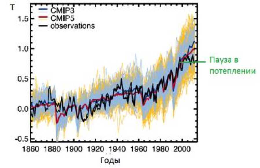
Figure 2. Global temperature (Т), calculated as per physical and mathematical models of the third-generation (CMIP3) and fifth-generation (CMIP5), and also real global temperature, resulted from observations for 1860— 2015 years [3]. Pause of global warming is marked with a green line.

According to opinion of IPCC, the unprecedented warming is expected by the end of XXI century. Figure 3 shows the trend of the expected climate change according to the IPCC version and the corridor of uncertainty of such forecast, resulting from the uncertainty of the model and the uncertainty of human impact on the greenhouse gases [2]. Figure 3 shows that the width of the corridor of uncertainty is 2 times more than the value of the forcasting increase in global temperature. The situation is similar for the regional forecasts, including the Arctic. Is it possible to make strategic plans for development of North on the basis of such uncertain forcasts? Gaps in deep understanding of some processes in the climate system and factors affecting it, are the main cause of significant uncertainty in predicting tends of climate cnanges using modern models. In such circumstances different approach is reasonable — the study of laws of the changes in climate variability, according to observations and their extrapolation.

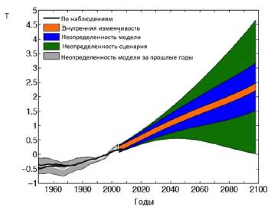
Figure 3. Forecast of global climate change trend as per IPCC version [3] and climate variability due to different reasons.

Dark line = observations. Orange = inner changes. Blue = uncertainty of a model. Green = uncertainty of a scenario. Grey = uncertainty of a model in past years.

Statistical model for the prediction of climate variability

Physico-mathematical models are desirable purpose of description of all physical processes in the climate system, but currently they are limited to insufficient knowledge of the physical processes and mechanisms responsible for oscillations climate variability. The search of the objective laws in time series of meteorological characteristics goes for a long time and not successfully enough. The lack of clear ideas about of the reasons of formation of fluctuations in atmospheric characteristics and unsuccessful experiences of search of objective laws in climate oscillations led researchers to hasty conclusions about the randomness of all processes in the atmosphere. Indeed, there no simple laws in nature, which for many years been the subject of research in the statistical analysis. For example, if the hypothesis about recurring disturbances in the time series appeared, then the accuracy of periodic processes was evaluated by the method of spectral analysis. At the same time for greater reliability of results in the analysis the maximum possible time series was used. As the result, statistically significant but systematically incorrect conclusion was received that the fluctuations in the time series are not periodic and it means that they are random. There were several methodic errors in this analysis. Firstly, repeating perturbances should not be necessarily periodic — it may be a series of interconnected perturbances in different time intervals. Secondly, even the periodic perturbances should not exist endlessly long while, as it is desirable to obtain reliable statistical estimates. Thirdly, periodic oscillations with imposing of additional factors may eventually change the sign or phase, their period can gradually stretch or shrink. For example, at the boundary of ocean-atmosphere inevitably slow changes of heat flux oscillation period occur together with changes in the thermal inertia of the upper layer of the ocean interaction with the atmosphere, and the inertia is changed depending on the changing thickness of the top layer of mixing and volume of the upper layer of water involved in the heat exchange.

By now, a lot of information is received about the behavior of the climate system, which implies the need to create other methods to find patterns and to make a statistical model.

The theoretical assumptions of the model. Global and regional climate on different time scales can be characterized by the change in its status and fluctuations. It should be noted that fluctuations in the atmosphere can be natural and forced ones and their properties are different. Free fluctuations are those which are made by the system near the position of stable equilibrium after the initial disturbance. The frequencies of these fluctuations are determined by the properties of the system and does not depend on the frequency of repeating impacts on the system. Free fluctuations occur only due to the internal forces to counter the initial disturbance (presence of a perturbing factor is required). This is the most important property of the independence of the natural frequencies of the fluctiations of the climate system from a period of external influences usually was not taken into account.

Forced fluctuations are those which happen under influence of the variable external forces. While investigating fluctuations, it is necessary to take into account that forced fluctuations have a frequency of disturbing forces, and free fluctuations have their own frequencies inherent to the system, and they are connected with disturbance only from the start time. This is the fundamental position to make a statistical model.

Atmosphere is the least inertial component of the climate system and that is why it is more readily reacts to external changes (impacts). Reaction of it is manifested across the spectrum of its own frequencies. The impact on the atmosphere of every disturbance from the different components of the climate system and external factors, every time is accompanied by starting a new series of its own disturbances in the atmosphere. Fluctuations on natural frequencies at every new startup have a new phase of the fluctuations (it fundamentally affects the method of allocation of periodicities). New fluctuations impose on dying out the previous ones. At the same time the interference, beats, etc happen. It is not always possible to separate periodic changes from them.

With all the complexity and multifactorial dependence of processes of the climate system, fluctuations in the atmosphere in some way are self-coupling, and there are rhythms that are easier to separate. The atmosphere has climatic memory for about two weeks, so long-term climate variations can not be accreditied only by vibrations at its natural frequencies. The longterm stability of the atmosphere is supported by other components of the climate system. The ocean can be hypothetically considered as possible nearest source of long-period rhythms which define a series of non-periodic disturbances in the atmosphere as a result of interference, beats and resonances. At the same time, we can not exclude other potential sources of direct rhythms in the atmosphere, such as irregularity of the angular rotation of the Earth, perturbations in the orbital motion of the Earth and other geodynamic factors and external influences.

The main source of knowledge about the climate system consists of observations and accumulated data sets of such observations. At any given point of time the original field parameters of the climate system, including the ocean, contains gradients, which in some initial point set the push to all system processes in the direction of levelling of gradients, like a pendulum, which was rejected before running from the vertical, and began to move. In this movement, the system as well as the pendulum, passes the equilibrium point by inertia and goes from equilibrium to the other side. Then the movement in the opposite direction begins, again towards equilibrium. In this way the initial gradients set dying fluctuations of the climate system on their own frequencies. The appearance of the initial gradients in the climatic characteristics of the system is always preceded by some external influence. The statistical model should extrapolate the moments of occurring of the external influences and coming after that sets of dying oscillations. Different components have different inertia, that is why fluctuations of different duration occur in the climate system. In the deep ocean processes and in the ice cover the periods of fluctuations can reach thousands of years.

Research of the rhythmic structure of the climate characteristics (primarily of temperature) on the basis of the data of the world meteorological observation network has allowed the author to make the statistical model of the regional climate, which coveres all regions of the Earth. Prognostic base of the model is the method of allocation of hidden periodicity, proposed by the author in 2007 [10, p. 14—26].

Model of periodical nonstationarity

In atmosphere, as well as in all non-linear systems, as a result of long-term external effects, short-period perturbations occur at the natural frequencies of the atmosphere. The superposition of several oscillations at the natural frequencies is manifested in the atmosphere as a series of disturbances which arise with apparent chaotic nature on the interval from one external action to another. With every forthcoming external influence, the whole series of seemingly chaotic fluctuations can be repeated. Such perturbations are called rhythmical. Rhythm is the alternation of any elements that occurs with a specific sequence. In nature there is polyrhythm. However, many of the rhythms in the climate system are weakly expressed and can be detected only with special analysis. During alteration of processes new dominant rhythms can arise which have never been before. The superposition of rhythms makes complex form of fluctuation values in the time series. Thus, statistical modeling should be directed to the description of the laws of long-term influences and to the description of free oscillations stepping after them at natural frequencies. In this problem formulation it is assumed that during model’s output there will be oscillations with frequencies different from the frequency of the external (relative to atmosphere) disturbances. It is assumed that after every external influence on the atmosphere a series of non-periodic disturbances in a certain strict sequence will arise (the result of superposition of vibrations at the natural frequencies). After each new external action in the atmosphere a series of new disturbances will occur, starting from the new phase.

From the statistical point of view, the forced fluctuations can be described by the model of the periodical nonstationarity (the terminology from [11]). Periodical forcing fluctuations in each period set a series of non-periodic forced disturbances.

It is widely accepted that [11] that the time series has a periodical nonstationarity if the whole series, and any of its segments are not stationary, but series is divided into such equal segments of duration τ, in which each value of meteovalue on one segment there is equal or near value through the τ units of time in the next interval:

t 1 ≈t τ+1 ; t 2 ≈t τ+2 ; t 3 ≈t τ+ 3 ; . . . t τ ≈t 2τ etc.

If periodical nonstationarity exists in the parameters of the atmosphere, then the temperature prediction task is to identify the period of nonstationarity τ – the period of forcing impacts. Forcing impacts on the atmosphere at regular intervals sets the rhythms for the series of fluctuation characteristics of the atmosphere on nature frequencies. In practice, the forcing powers are truly unknown. According to meteorological observations we have only series from the superposition of natural oscillations of complex shape. And according to these series of disturbances it is necessary to allocate the period τ of hidden forcing rhythm-making fluctuations.

If τ is known, then time series can be divided into intervals with duration τ, where τ is the period of forcing fluctuations. That is if we know τ, series can be divided into a few intervals in such a manner that every member of series ti will be equal or close member ti+τ, where τ is the period of forcing impacts. The series of values t1, t2, … tn of meteorological value (temperature) can be of any complexity – periodical or non-periodical with variable phase and amplitude.

τ period must be found empirically, through all its possible values by checking the similarity of disturbances in neighboring segments of the time series. In general, the work begins with the search of period τ of the repetition of a series of non-periodical perturbations of meteorological values, which are the result of forcing impacts. As a rule, rhythms in the atmosphere can be traced 23 times and then are washed out, so testing is done at the last interval of the time series of observations lasting 3T in total. Other data is not used at this stage. The elements of this seriesinterval will be values from t1 to t 3τ . In every tested value of τ analyzed series is divided into three segments with τ duration. If number 1 is to identify the first element of series t, and increase the number by 1, the following segments of series of elements will be received: the first segment — t 1 to t τ , the second segment — from t τ +1 to t 2τ , the third segment — from t 2τ+1 to t 3τ . The meaning of t 3τ is the last member of series of observations. According to the first and second periods of time the average etalon of the temperature perturbation on the test interval of time duration τ is calculated. The meanings of this etalon are:

T i =(t i + I t +i )/2; T 2 =(t 2 + t T +2 )/2; T 3 =t + t т +з )/2 etc. to T t = (1 т + t₃ T )/2 .

The temperature changes t , on the third (last) time interval were compared with the Ti changes T , in the received tested etalon ( i = 1, t ). Their similarity was estimated by the correlation coefficient. After similar calculations for all possible test values of τ, the duration of the interval T was determined, in which the similarity of changes in the first segment and in the tested etalon was maximum in value of the correlation coefficient. If the best correlation coefficient is statistically correct, then according to the hypothesis of rhythms, the period τ — is the time through which a series of non-periodic oscillations is repeated on the interval τ. At that the entire complex overall picture of fluctuations becomes predictable for τ values in advance. Isolation and extrapolation of the rhythms is the essence of the statistical climate model.

In practice it turned out that the allocation of one meaning τ is not enough. A lot of different factors with their system of rhythms affect the regional air temperature. The set of these rhythms varies depending on the season, circulation, physical-geographical and other conditions. Therefore, multiple search of rhythms is arranged and such a set of rhythms is selected that describes in the best way the temperature change for the years, prior to the last forecast.

Each forecast is based on the rhythms allocated for the particular station and month. Sets of rhythms are different. Preliminary analysis showed that in January the rhythms of 5, 13, 18, 35-

37 years dominate at the stations of Russia, in December — 8, 11, 18 and 35-37 years, in other months, as a rule, 5-6 rhythms in range 3-18 years occur. 18-year rhythm has the highest frequence in January, July — August, in September — October, and in December, it is sometimes changed by the strong rhythm of 17 or 19 years. In cases when there is no 17-19-year rhythm, there is 16-year rhythm, it usually happens in the first half of the year. 10-11 year rhythm in all manifestations corresponds to 10-11-year cycle of the solar activity. The rhythm of 10-11 years can be traced only during cold half of the year. It is a well known fact described in the literature—the solar-atmospheric connections are more resistant during cold half of the year. Increase of the frequence of the 11-year rhythm in March — April is in line with the known fact that during these months, and in October-November the favorable conditions of interaction of the geomagnetic field with the interplanetary magnetic field in which the invasion of solar corpuscles in the Earth's atmosphere become easier with strengthening solar activity. 8-9-year rhythm for stability is similar as 18-year cycle, sometimes (in June and August), 8-9-year rhythm is replaced by 7-year one. Both these rhythms coincide with the features of the interaction of the Earth and the Moon. 4-year rhythm sometimes turns into 3- or 5-year rhythm.

Basing on duration of mentioned rhythms the hasty conclusion can be made that by chance any rhythms can be allocated in range 4-18 years or more. In fact, the state of the climate of any particular month of the year is described by some limited coherent ensemble of rhythms, the duration of each can vary slightly over the years. The ensemble of rhythms is always not much different from the set of 4-6, 8, 11, 18, 35 years whose origin is to be studied. A wide variety of rhythmic wave motions in the atmosphere is stipulated by the influence of forces of different origins.

So basing on the analysis of these observations of climate variations, the author formed a new idea at the properties of the natural oscillation characteristics of the climate system, and the statistical model of hidden rhythms in the atmosphere and their subsequent extrapolation in time is developed. Research of forecast air temperature values with this model showed that the model allows us to make prognostic assessments of climate fluctuations 2 decades in advance.

Forecast success rate of climate fluctuations

The above mentioned pause in warming of the global climate since XXI century, which was not predicted by the best physical-mathematical models of the climate. In fact, based on the statistical model, delay of the global warming was predicted already in 2007. The forecast was published in printed form in the monograph [7] (available on the website and in the abstract of the author's thesis [12].

Chapter 7 of the monograph [7] dated by 2008, shows that on the basis of extrapolation of natural rhythms the delay of warming is expected in interval till 2025. Figure 4 depicts a predictive temperature graph, which was published in 2008. In the chart the trend line showed the expected pause in warming, bold curve — the forecast of year-by-year temperature changes. Now the forecast can be evaluated.

The best independent test of the accuracy of the forecast of the climate change is the comparison of the previously published forecast with new data of observations. Such opportunity was received — the forecast till 2025, published in 2008 in the monograph, in the abstract of the thesis and on the official website "Russian Research Institute of Hydrometeorological InformationWorld Data Centre" (RRIHMI-WDC), this forecast was compared with observational data published at NASA website in January 2016. The forecast was made in 2007 on the basis of observational data until 2006. Calculated on the base of the author’s model, the trend of delaying of warming was completely confirmed in the interval of 2007—2015. The pause is highlighted in Figure 2 as per modern observations and in Figure 4 as per forecast made in 2007.

Besides, the comparison of year-by-year forecast and actual values of the temperature in the interval 2007—2015 showed the matches of the major peaks of anomalously warm years 2009— 2010 and 2015, as well as match of conditions during less warm 2008, 2011-2013.

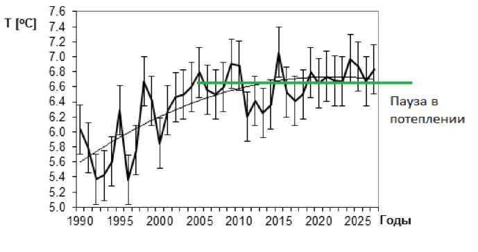
Figure 4. The average annual air temperature of the northern hemisphere based on observational data for 1990-2006. and the author's forecast for the period 2007-2025 gg. (from publication of 2008 [8, 13]).

The diagram (Figure 5) shows the actual temperature values of the northern hemisphere (Тн) according to NASA for the period of 1961—2015 and published in 2008 prognostic values of the air temperature (Тп) for the period of 2008—2025, obtained by the author’s statistical model.

Тн

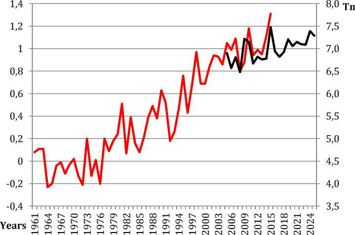
Figure 5. The average annual temperature over the continents of the northern hemisphere of the Earth: the forecast from [8, 13], made in 2007 for period of 2007—2025. (Тп) and the actual temperature values as per observations at meteorological stations in the northern hemisphere [16] till 2015 (Tн)

Comparison of the forecast values with the actual data showed that the on the interval of the first decade of forecast, the statistical model allowed us to predict all the basic features of interannual fluctuations of the average climate of the northern hemisphere and the long-term warming trend of the warming delay in the northern hemisphere of the Earth at the beginning of XXI century. For comparison it should be pointed out that the best physical-mathematical climate models did not predict warming delay at the beginning of the XXI century they are not intended for forecasting of interannual climate variability. In the basis of the described model there are new ideas about the structure of fluctuations in regional climate and observation data from 8,000 stations of the northern hemisphere. The model allows to calculate the expected climate changes with quantitative estimates for each meteorological station of the Earth.

Seasonal and monthly weather forecasts with a year lead- time

The theoretical suppositions mentioned in the section about forecast of climate variability, were suitable also for the shorter time scale prediction of the air temperature and elements. Seasonal and monthly forecasts with one-year lead- time turned out to be successful.

Despite the smooth progress of the annual average daily insolation, the general circulation of the atmosphere keeps throughout the season the main directions of main air flows and the position of the centers of atmospheric actions, and then suddenly switches to another mode corresponding to the next season. One can figuratevly say about this known fact that the atmospheric circulation can be quantized according to seasons. The ability of atmospheric circulation to be quantized seasonally is well known, it is usually referred to as the atmospheric circulation ability to abruptly switch from one mode of circulation of one season to different mode, specific for the next season, the essence remains the same. The second example of quantization is the circulatory era — it is the largest stage of the process of the development of the atmospheric circulation with a specific character of interannual and annual microtransformation of circulation, formation and distribution of thermobaric fields in the hemisphere.

For a long time, seasonal forecasts were based on the analysis of succession of atmospheric circulation types from season to season. Asknaziya A.I. [16] wrote in 1936: "Can we assume that approximately the same conditions of hydro, litho- and atmosphere in one season will lead to approximately the same conditions of the next season, or on the contrary, ... close initial states can… lead to completely different weather patterns. If the first assumption is correct, then sooner or later the problem of the long-term forecast will be solved. If the second is correct, then you need to have courage to say openly that the problem of long-term forecasts is, at least in our time, insoluble." Until recently, such a philosophy of prognostic ties remained. Now it is clear that such arguments are not quite correct.

One of the reasons of the lack of the quality of the long-term forecasts may probably be neglect of quantization of the atmospheric circulation features seasonally, spacely and rhythmically over the years. Despite the fact that within the year inter-seasonal connections are very weak, while for the month forecast special importance was given to the data for the last month or decade. The forecast of the average air temperature for coming month was usually based on an extrapolation of the atmospheric processes, immediately prior to the forecast. In fact, succesfull approaches were used to the methods of long-term forecasts, taken from the experience of the creation of short-term and medium-term forecasts. But lead-time of the forecasts with this approach was limited by one month.

Weather conditions in the region are determined to a large extent by the type of coming air mass. Tradewind zones of northern and southern hemispheres are served as centers of formation of the tropical air, limited by belts of subtropical anticyclones in both hemispheres. Polar air of the northern hemisphere is formed in the Arctic and sub-Arctic regions and the polar air of the southern hemisphere is formed in the Antarctic and sub-Antarctic regions. The air of the moderate latitudes occupies the space between zones of polar and tropical air. Air masses are different not only in values of the meteorological elements but also in factors of forming, with a different set of cyclical components and various statistical and prognostic properties.

Seasonal differences in the atmospheric circulation of the moderate and high latitudes create a kind of oscillation frequency filter. This filter differentiates fluctuations depending on the proximity of a period to the value divisible the duration of one year. Oscillations with even period of years have advantages in comparison with the periods of the other values. Fluctuations with periods aliquant to year are transformed into long-period perturbations. External influences on the atmosphere with periods Т1 aliquant to year, can be manifested in the extratropical latitudes with periods Т with n times longer than the initial tropical disturbances: T = nT1, where nT1 — integer number of years with minimum integer of n.

Thus, basing on the known properties of atmosphere, it is clear that long-term external impacts to atmosphere can lead to one type weather changes of the extratropical latitudes only in the corresponding seasons, under identical seasonal conditions of the atmospheric circulation. External cyclical impact on extratropical atmosphere is possible only at certain frequencies divisible to one year or in time interval nT. This means that the impact with the period, for example, of two years will be manifested in the atmosphere in 2 years; impact with the period of 2.5 years will be manifested in the atmosphere of the similar season only in 5 years, and impact with a period of 2.2 years — in 11 years etc. The availability of the peculiar frequency filter results in situation when the fluctuations with frequencies of the forcing oscillations are not detected in the atmoshere, but the rhythms occur with intervals of several times greater than the periods of forcing fluctuations. For example, if in the ocean depths there is a cycle with the period of 18 months, then it will be manifested in extratropical atmosphere not every 18 months, but only in 3 years (36 months), similarly, cyclic impact with the period of 20 months — will be manifested only in 5 years (60 months), etc. Bearing in mind this seasonal filter it is not possible to expect that approximately the same conditions of hydro, litho- and atmosphere of one season will lead to approximately the same conditions of the next season. But it is possible to find patterns of occurrence of rhythms, divisible to one-year period, and a series of disturbances in the atmosphere following for each rhythm. Frequency of one year cycles automatically gives lead-time of the forecast starting from one year. This approach was used in the author's method of seasonal and monthly temperature and precipitation forecasts with lead-time of one year.

To check the quality of forecasts of air temperature anomalies including its sign and value following method published in [17] was used as described in the guidance document2. According to [17], the quality of the forecast is considered satisfactory if its error is less than the climate forecast error. The forecast can be satisfactory only as per the sign of anomalies, satisfying only in the deviation from the actual level or satisfactory as per two of the indicators. In the latter case, the quality of the forecast is accepted as good. If none of the terms of comparison with climate forecast is not fulfilled, then the forecast is taken bad.

The essence of evaluation as per "value" is that forecasts are considered to be satisfactory in which the standard error is less than the natural variability of the series. It means that satisfactory forecast can reduce the uncertainty of our knowledge of coming meteorological values. Calculations of evaluations of the quality of the had been conducted by the author's forecasts for 400 stations in Russia for 10 years. 400 evaluations were received for each month, each season and year. Based on these evaluations, the number of stations was calculated in % with different quality of the forecasts of temperature anomaly in three variants: a) match of actual and prognostic anomaly in sign and value; b) match in sign; c) match in value. In all variants the total number of stations — 400 was taken as 100%. The sum of the evaluations of three variants for month can exceed 100%, as the evaluations as per variants are calculated independently. The number of stations with "good" and "satisfactory" forecasts are shown in the table 1 and 2.

Table 1

The number of stations (%) with "good" and "satisfactory" forecasts of anomaly of the monthly air temperature

Suitability mark	I                   II		III	IV	V	VI	VII	VIII	IX	X	XI	XII	Averag e
а) In sign and value	55,7	45,3	28,8	11,4	19,6	22,5	29,8	22,8	34,2	25,3	31,0	5,7	27,7
b) In sign	76,3	72,5	66,8	59,5	58,9	55,7	80,1	72,5	73,7	71,2	57,9	30,7	64,6
c) In value	71,8	63,6	44,6	27,2	25,0	30,7	36,1	28,8	39,9	33,9	42,4	25,0	39,1

Table 2

Forecast success rate (%) in sign and value of anomaly of the average season and average annual air temerature

Suitability mark	Winter	Spring	Summer	Autumn	Year
a) In sign and value	96,2	66,1	74,1	67,4	90,2
b) In sign	96,5	73,4	86,7	72,2	90,2
c) In value	98,7	90,5	86,1	84,5	97,0

Estimates detailed per months (Table 1) show that the forecast success rate of monthly temperature is always better in sign than in value. Forecasting method has smoothing properties, the sign of anormaly is often predicted correctly, and the value is understated. Better quality of forecasts is observed in January — 76.3% of the stations with forecasts satisfactory in sign and 71.8% — in value, and also in July — satisfactory forecasts in the sign were at 81.1% stations. Forecasts satisfactory in sign on more than 70% of stations were observed in January — February and in July — October. During other months there were less stations with satisfactory predictions.

According to summarized estimates for all months, it turned out that on the average in Russia at 24.0% of stations the forecasts of the average month temperature were poor, at 64.6% of stations evaluations showed satisfactory forecasts in sign of average month anomalies, at 39.1% of stations satisfactory forecasts in value of anomaly were observed, and at 27.7% of the stations the predictions were good both in sign and value.

Forecasts of average seasonal and annual avalues were more accurate (Table 2). Such predictions were satisfactory in sign or in anomaly value more than at 70% of the stations. Better quality of forecasts was in winter (more than 90% of the stations with good forecasts) and in summer (over 80% of the stations with good forecasts). In the spring and autumn about 70% of stations with satisfactory forecasts in sign, and 84-90% of stations with satisfactory predictions in value. While forecasting the average seasonal values, the negative smoothing method properties are not manifested, as the series of actual average seasonal temperature values are more smooth and probably more amenable to statistical modeling. There were about 96% of stations with good seasonal forecasts in sign and value in winter, 74% in the summer, and in spring about 66%. Average annual values are predicted well at 90% of stations (Table 2).

The price of forecast of the climate change of the Arctic

Significant changes in the characteristics of the ice cover in the Arctic [18, p. 814—818; 19, p. 59—65] open new economic prospects for the development of resource-rich Arctic shelf rich and for sea transportation of goods along the Arctic coast of Russia. Life and human activity in the Arctic is much complicated by severe climate conditions. Transportation of life-supporting cargo in the Arctic is only possible on the open water during periods of low ice concentrations in northern seas away from the multi-year ice. The seasonal sea ice cycle affects the human activities and life environment of biological species. In recent years, sea ice area decreased [13; 14]. Ice melting in the Arctic Ocean in summer gives the access to fossil energy sources in the shelf zone. This contributes to the development of the Arctic.

Current plans of the Arctic exploration and extraction of mineral resources technology are built on the assumption of expected continuation of global warming. But there is great uncertainty regarding climate forecast. In the case of climate cooling new technologies of subglacial exploitation will be required.

Nowadays for the development of the North a new transport system is needed. It is already planned to create in the north of Siberia the transport system with access to Northern Sea Route. The main drawback of Northern Sea Route — period of navigation there is possible for 2-4 months a year in conditions of today's abnormally warm climate. In the case of climate cooling Northern Sea Route will be lost.

Even today huge funds are invested in the development of the Arctic. Hoping that warm climate will be preserved, at Yamal Peninsula Sabetta port is under construction now. It is planned to build 700-kilometer railway line from the south to port Sabetta. Plans for building of new supporting Arctic port at the Barents Sea coast near Indiga Bay are considered. It is also planned to build liquefied natural gas plant, terminals for large tankers, oil terminals, to provide a basis for minor ship repair.

It is important to know whether the climate conditions of the future meet today's technology of extraction and transportation of mineral resources in the North. The future of the North depends largely on the future climate.

Conclusion

The severe climate of high latitudes is a limiting factor of the development of the north. Current warming has become favorable for the development of mineral resources on the continental shelf of the northern seas and for the use of Northern Sea Route as a major transport way along the entire northern part of Eurasia.

Based on the climate system observations and long-term research of fluctuations of the climate system as well as external disturbing factors, new ideas about the structure of the fluctuations and the laws of appearance of rhythms in the characteristics of the atmosphere were described, which made it possible to make the statistical model of air temperature fluctuations basing on new principles. The statistical model allows to obtain new prognostic evaluations of climate change for the next two decades. The regional temperature values are predicted as per observation points, in small and large regions. This model is multifunctional and can be applied to any region and for different characteristics of the climate system.

Model has been taking copyright test since 2007. The pause in global warming observed since the beginning of XXI century has been predicted by the model in advance before the reveal of the pause (the forecast for each year up to 2025 of the average annual air temperature in the northern hemisphere was published in 2008).

Interannual variations of climate anomalies forecasted in 2008, coincided in sign with year-by-year values of temperature anomalies of the next observations up to 2015. Abnormally warm 2009—2010 and 2015 were forecasted (above trend values), and also less warm 2008, 2011— 2013 (below trend values).

The prognostic model for seasonal and monthly air temperature forecasts and amount of precipitation for one year in advance has been developed with including of the seasonal features of transformation of the rhythms. Estimates of the quality of forecasts made on independent data, have demonstrated their informational content.